University of Twente
EEMCS / Electrical Engineering
Control Engineering
Simulation with Hamiltonian mechanics
Creating a module for 20-sim
Eric Staal
MSc Report
Supervisors: prof.dr.ir. J. van Amerongen
dr.ir. P.C. Breedveld dr. N. Ligterink ir. B.P.T. Weustink
January 2007
Control Engineering
Summary
The simulation program used and developed at the university of Twente, 20-sim, is using simple spatial models for simulation. The spatial models used in 20-sim do not allow simulation of realistic effects, like resonating frames, bending and breaking of beams. To model these structures 20-sim need to be extended to simulate these effects.
This can be realized by making a module for 20-sim which is able to model these effects. Modeling these structures and effects can easily be modeled using Hamiltonian mechanics. Hamiltonian mechanics have a different approach in comparison to classical, Newtonian mechanics. How Hamiltonian mechanics are used is described in this report.
The assignment is to create a module for the simulation program 20-sim which is able to model realistic effects using a continuous spatial description with Hamiltonian mechanics. This module consists of two parts. The main application is necessary to input models, change models and to draw the model. This application is used to set up the simulation parameters. The actual simulation is done by second part of the program. This part is called by 20-sim to do the simulation with the model made with the main application.
Several models are tested to see if the add-on module could simulate Hamiltonian models correctly. The results gave useful information. Most of the testing results are as expected and most results could be explained. However some results are unexpected. Further testing has to be done to see where these unexpected effects come from.
The assignment has several recommendations. The interface which is used in the main application is only able to model simple Hamiltonian models, models which consist of point masses and stiffnesses. To make the application work with other types of Hamiltonian models some changes need to be made. Secondly the integration method used is quite simple. This resulted in simulations becoming quickly unstable. This can be solved with small integration steps to stop the model from getting unstable.
Samenvatting
Het simulatie programma wat de universiteit van Twente gebruikt, 20-sim, gebruikt eenvoudige ruimtelijke modellen om de werkelijkheid te simuleren. Deze modellen zijn vaak voldoende om alles correct te simuleren. Echter zijn er sommige aspecten die wel in werkelijkheid voorkomen maar dan niet gemodelleerd kunnen worden. Hierbij kan gedacht worden aan resonerende frames, doorbuigende balken, et cetera. Dit is met 20-sim moeilijk te modelleren. Om dit soort realistische effecten wel te kunnen modeleren moet 20-sim uitgebreid worden zodat deze realistische elementen wel gebruikt kunnen worden.
Dit kan gerealiseerd worden door het simulatieprogramma uit te breiden met een module om deze ruimtelijke modellen te simuleren. Dit kan eenvoudig worden opgelost door Hamiltoniaanse mechanica te gebruiken. Hamiltoniaanse mechanica heeft een andere aanpak dan klassieke, Newtoniaanse mechanica. De Hamiltoniaanse mechanica zal worden uitgelegd in dit verslag. De opdracht is een module te maken om het simulatieprogramma 20-sim te laten werken met deze Hamiltoniaanse mechanica. De module moet in staat zijn om modellen te laden en te simuleren op basis van Hamiltoniaanse mechanica. Deze module bestaat uit een tweedelige applicatie. Het
hoofdprogramma wat noodzakelijk is om modellen in te voeren, te wijzigen en te tekenen. Het andere deel wordt gebruikt om de simulatie uit te voeren met 20-sim.
Enkele modellen zijn getest om te kijken of het resultaat voldoende was. Het resultaat bleek veel aspecten te hebben zoals deze ook in de realiteit voorkomen, echter waren er ook dingen die onverklaarbaar waren. Deze onverklaarbare aspecten moeten nog nader onderzocht worden om te kijken waar deze vandaan komen en of ze te verklaren zijn. Hieruit kan dan de conclusie getrokken worden of het een simulatie- of modelfout is.
Het programma bevat nog een redelijk simpele interface, er zijn maar een aantal basis Hamiltoniaanse modellen die gebruikt kunnen worden. Om het programma met meer modellen te laten werken zal het programma aangepast moeten worden zodat ook andere soorten modellen, dan modellen met
Control Engineering
Table of contents
1 Introduction ...1
1.1 Assignment ...1
2 Hamilton function ...1
3 Creating a plug-in for 20-sim ...8
3.1 Choices for tooling...9
3.1.1 Connecting Hamiltonian mechanics to 20-sim...9
3.1.2 Communication between the DLL and the host application ...11
3.1.3 The integration method...14
3.2 Design ...15
3.3.1 Storing the Hamilton ...16
3.3.2 The derivative of the Hamiltonian...17
3.3.3 Synchronizing the drawing...19
3.3.4 Storing the model ...19
3.4 Results...20
4 Model testing...25
4.1 Static models...26
4.1.1 Poisson’s ratio ...26
4.1.2 Clamped beam with a force ...29
5 Conclusion and recommendations ...59
5.1 Conclusion ...61
5.2 Recommendations...61
Appendix A: Glossary ...63
Appendix B: Example static DLL ...63
Appendix C: Dynamic DLL struct ...64
Appendix D: SFunction cases...64
Appendix E: Example dynamic DLL ...65
Appendix F: Class diagram ...67
Appendix G: Shared memory struct ...68
Appendix H: Calculating total energy ...68
Control Engineering
1 Introduction
When trying to model a real world spatial situation, restrictions are made to get a simplified version of the real world. However, sometimes the restrictions which are made have a bad influence on the model so it does not match the real world sufficient enough. To make a more realistic spatial model, the model will become more complex. Models with a continuous spatial description are therefore harder to simulate.
With conventional simulation techniques it is hard to simulate when a piece of material goes from bending to folding or even breaking. When a piece of material is modeled as a linear model it only works for a maximum deflection, when the force and so the deflection gets too big the linear model is not sufficient enough and another model have to be chosen. Therefore a solution needs to be found which makes it possible to simulate these non linear effects and not only the linear effects for small deflection.
A solution can be found in the form of models based on Hamiltonian mechanics. These mechanics allow creating non linear models. 20-sim, a simulation program developed by the University of Twente, does not have an out of the box solution for creating more realistic models for spatial
situations with non linear effects, as bending, stretch and shear, therefore a module needs to be written to make these more realistic models for spatial situations work with 20-sim.
1.1 Assignment
The assignment is to write a module for 20-sim which describes a non-linear Hamilton function. A Hamiltonian describes the energy function of a system. This system can have single or multiple in- and outputs. Each input and output is connected to other parts of the model without generating or wasting energy, this is called power continuity. The transportation of energy to and from the
Hamiltonian model is realized with two power ports. Each power port is described by an effort and a flow. The total transferred energy per port is the product of these two terms.
The begin situation is the code written by N.E. Ligterink. This code is written without an user interface as a stand alone application. The assignment is to make this code work with 20-sim and to give it an user interface. To solve this assignment some background information about Hamiltonian mechanics is needed, this is described in chapter 2.
The assignment consists of several subparts:
The construction of the Hamiltonian should be done automatically. The Hamiltonian must be constructed for several basic parts, these parts are a bar, a plate and a block. These parts can have different kinds of energy: bending, stretch, and shear.
Constructing the state vector. The state vector must be initialized at the beginning of the simulation and it must be possible to read this state vector in and out. This makes it possible to change the state vector to a desired position and to read out the current states.
An interface with 20-sim is also necessary. This interface must set down the port variables and the causality, so other models can be connected to the Hamiltonian model. The interface influences the state vector, so it is possible to change the state vector while it is operating.
The last part is the simulation of the system dynamics. The system dynamics are shown by doing a time integration which cooperates with the 20-sim simulation. The system dynamics have to be shown in a graphical interface which has to be time dependent.
University of Twente
2 Hamilton
function
In this section some background information is given about Hamiltonian mechanics. This information is needed to understand the assignment.
Each system has a specific energy function which describes its dynamic behavior. The energy of a system can be described with a Hamiltonian. First some explanation about the Lagrangian is given to understand the Hamiltonian. The Lagrangian describes the equations of motion of a system. The Lagrange equations are a reformulation of classical, Newtonian mechanics. The Lagrange equations are introduced in 1788 by Joseph Louis Lagrange. The trajectory of an object is derived by finding the path which minimizes the action, a quantity which is the integral of the Lagrangian over time. The Lagrangian for classical mechanics is taken by the difference between the kinetic co-energy and the potential energy.
The Lagrange equations simplifies many physical problems, because there are less equations since it is not directly calculating all the forces but only the force which minimizes the action. Therefore it would be possible to calculate more complex systems with less calculation.
Two examples of dynamic systems are shown below. The first system is a simple pendulum. The pendulum swings until all mechanical energy is disappeared due to friction. This pendulum is used in many mechanical systems, i.e. a clock and it easily can be modeled with Hamiltonian mechanics. The second picture, of a crane, must handle large masses without bending or breaking. The machine must be that strong to hold a heavy load. Bending of the crane can be modeled to test if the crane is strong enough to hold a certain load. Dynamic effects like a vibrating frame also can be modeled.
Control Engineering
Figure 2: Drawing of a crane
When these systems are modeled with Lagrange mechanics the results can be obtained with less calculation than with classical mechanics, therefore the results are obtained quicker. Lagrange mechanics are used to calculate the path which minimizes the action.
The independent variables of a Lagrangian are
q
andq
.q
are the generalized coordinates andq
the generalized velocities. The Lagrangian is a function ofq
,q
and the time which can be written asL T= ′−V
Where L is de Lagrangian, T’ is the kinetic co-energy and V is the potential energy, the latter two expressed in the generalized coordinates. In order to express the kinetic co-energy and potential energy in generalized coordinates, commonly a coordinate transformation is required that reduces the number of generalized coordinates to the number of degrees of freedom. If this cannot be done
straightforwardly, for instance by means of symmetry considerations, additional constraints have to be added by means of the so-called Lagrange multiplier.
If not all the forces acting on the system are derivable from a potential, then Lagrange's equations can be written in the form
j
where the first term represents the rate of change of momentum, the second term the conservative forces and the last term the non-conservative forces.
The generalized coordinates used in the Lagrangian can be useful, below an example is described where the use of these generalized coordinates is made clear. When a point mass is moving in a plane, it has two degrees of freedom, X and Y in Cartesian coordinates or angle and radius in polar
University of Twente
coordinates, there are still two degrees of freedom, X and Y. This is a rather simple example where the use of generalized coordinates is useful. When a model gets more complex the generalized coordinates may have even more advantage.
Lagrangian mechanics result in a set of second order differential equations of which numerical integration is difficult. In a bond graph representation this is demonstrated by the fact that all kinetic storage ports are written in differentiated causality. This means that the equations are not written in a form that can be numerically integrated in straightforward manner. This will require additional processing power.
Another way to obtain the equations of motion of a model is with Hamiltonian mechanics.
Hamiltonian mechanics look a lot like the Lagrangian mechanics but has a few differences. In a bond graph representation all kinetic ports remain their preferred, integral causality, which means that the true energy, i.e. the sum of kinetic and potential energy called Hamiltonian is a function of the generalized momenta and generalized coordinates. The Hamilton is thus defined as
H T V= + ,
where H the Hamiltonian, T the kinetic energy and V the potential energy. Note that this is the expression for the total energy, T+V. This is no accident, but a general property of natural systems. The generalized momentum is related to the Lagrangian as follows:
j
This means that a Legendre transformation is required to change the generalized velocities as
independent arguments of the Lagrangian into the conjugate generalized momenta as the independent arguments of the Hamiltonian:
(
j,
j,
)
i i(
j,
j,
)
i
H q p t
=
∑
q p
−
L q q t
= +
T V
In the example of the point mass in a plane mentioned earlier both the Lagrangian and the Hamiltonian are calculated and the role of the generalized coordinates is shown. First the model is described in Cartesian coordinates. The figure of this model is shown in Figure 3.
Figure 3: Moving particle in Cartesian coordinates
The particle is represented by the point p and has a mass m. Point p has an X and Y coordinate to represent to location of the point is the plane. The momentum of this particle is described with
x
The Lagrangian for this system is
2 2
1
1
( , )
2
2
Control Engineering
The Hamiltonian and Lagrangian are for an unconstrained model. When the radius is fixed, so
2 2 2
Both functions still have two terms. The constraint has not resulted in a function with fewer terms. If the same model is described with generalized coordinates, polar coordinates in this case, it can be seen that the function will only have one term left, instead of two.
In Figure 4 the same model is shown with polar coordinates.
Figure 4: Moving particle described with polar coordinates
The polar coordinates are described by an angle, θ, and a radius, r. When using polar coordinates the generalized momenta are given by
2
The Lagrangian for the unconstrained motion of p in the plane is
( )
Thus the Hamiltonian for this motion is
(
)
1
21
2 2( )
This can be simplified into
( )
When the particle only rotates around the center with a fixed radius, the momentum in the r direction,
University of Twente
The constraint resulted in a Lagrangian and Hamiltonian with only one term. Both functions became simpler because of the generalized coordinates. So when the generalized coordinates are chosen correctly it can result in fewer terms in the Lagrangian and Hamiltonian.
The Hamiltonian is used to describe the Hamilton’s equations. These equations are a set of 2n first-order equations. Lagrange’s equations are a set of n second-first-order equations. n is the number of variables in a model.
The first pair of Hamilton’s equations for the model described in polar coordinates is
2
They simply reproduce the relations between velocities and moment. The second pair, is
2
These relations combine Newton's second law with the fact that the conservative forces are the partial derivatives of the total energy with respect to the displacements. Because the Hamilton’s equations correspond to an integral causality in a bond graph representation, these equations can be solved numerically in a more straightforward manner than Lagrange’s equations.
In the constrained model where the radius is fixed and the potential energy is zero, so Pr is 0 and the
velocity in the r direction also is 0, the Hamilton’s equations are
2
The generalized coordinates caused Hamilton’s equations to be simplified. The term
p
r is not zero because there is still centrifugal force working on the rotating mass.With this example the advantage of generalized coordinates is given. The module which is written for 20-sim, must model all kinds of models. One set of coordinates is used, because it is very hard to change the coordinate system for each model. Cartesian coordinates are the most common type of coordinates and therefore they will be used in the module. This can result in large equations, but this should not be a problem because the equations are solved with a computer.
Another example is a girder modeled with several nodes. A normal girder will look like the picture shown below.
Control Engineering
This girder can be modeled in a 2-dimensional way by making several pieces with a mass and a stiffness between each other. If this girder is modeled as point masses with stiffnesses between them a model as shown in Figure 6 is obtained.
Figure 6: Girder modeled with nodes
Each node is on a fixed position and is held together with the stiffnesses. This girder is modeled as a 2-dimensional model, therefore it is a simple model of a girder.
Each dot is modeled as a node and each line as a stiffness. In this configuration the Hamiltonian (without gravity) looks like:
And the Lagrangian looks like
2
Each X represents the coordinates of each node, k is the stiffness between the nodes and d is the rest distance for the stiffness. Each node has 2n states, where n is the dimension. n of them are for the position and the other n for the momenta. With these 2n states it is possible to calculate the Hamiltonian.
This kind of model is the point of departure for further models. Each model will be described as point masses and virtual stiffnesses. This makes it easy to create models which are sufficiently competent within the problem context.
The model is not a stand-alone model but has connections to other parts. All the parts make one complete dynamic system, e.g. a crane, a printer or a car. To connect a subpart of a model with other parts of the model the so-called port concept is used. The port concept uses a connection between energy storage elements which has power continuity. This means that no energy is generated or wasted in the connection. Each connection, power port, transfers an energy P. P is represented by the product of effort and flow.
University of Twente
Both types of storage elements have another definition of effort and flow. For a q-type buffer these definitions are:
flow
v
dx
effort
F
kx
dt
= =
= =
.A p-type of storage element has the effort and flow defined as:
flow
v
p
effort
F
dp
m
dt
= =
= =
.With the effort and flow defined the energy for both storage elements can be defined:
2
The Hamiltonian model can be defined as a p-type or q-type storage element. This depends on if a force or velocity is applied to the model. When an effort (force) is applied to the system a velocity is returned. The force or velocity can be practiced on one separate node or on the whole system. This can be seen as a bowl where the model is lying in. This bowl is represented by a mass less point which has a stiffness connected to each point mass in the system. So when this bowl, the mass less point, is moved all other nodes undergo a force or a velocity.
More about the coupling of the Hamiltonian to other parts can be found in section 4.
All the information about the Hamiltonian and Hamilton’s equations is necessary to understand the problem context and to make correct design decisions. In the next chapter the design of the module is given.
More information about the Lagrangian and Hamiltonian can be found in (Lagrange, 2006),
Control Engineering
3 Creating a plug-in for 20-sim
To make 20-sim (20-sim, 2006) work with models with a continuous spatial description a plug-in needs to be written. This plug-in makes it possible to model these spatial models within 20-sim. This chapter describes all steps which are taken to make 20-sim work with Hamiltonian mechanics and how the module is designed and created.
3.1 Choices for tooling
This part describes several choices which led to the actual program. Each step is described carefully and all decisions are explained.
3.1.1 Connecting the module to 20-sim
There are two ways to connect an external simulation module to 20-sim. Both methods are described and the conclusion is mentioned below.
3.1.1.1 Static DLL
The first method of connecting a third party simulation application to 20-sim is by using the ‘static DLL’ functionality of 20-sim. The static DLL (Dynamic Link Library) functionality uses an external DLL, written in any source code, to obtain a result from a given value. The DLL can be written in any programming language if there is a simply input-output function in it.
An example of the static DLL functionality is shown below:
parameters
string filename = 'example.dll'; string function = 'myFunction'; variables
real x[2],y[2]; equations
x = [ramp(1);ramp(2)];
y = dll(filename,function,x);
In this example it can be seen that the external DLL has the name ‘example.dll’. The function which is called every integration step is ‘myFunction’. So the DLL should have a method which has the name ‘myFunction’ which must return a value when two variables are given. The input in this example is a one-dimensional array with two values, ramp(1) and ramp(2).
The user-function in the DLL must have certain arguments. The function prototype is like this:
int myFunction(double *inarr, int inputs, double *outarr, int outputs, int major)
where:
inarr pointer to an input array of doubles. The size of this array is given by the second argument. inputs size of the input array of doubles.
outarr pointer to an output array of doubles. The size of this array is given by the fourth argument. outputs size of the output array of doubles.
major boolean which is 1 if the integration method is performing a major integration step, and 0 in the other cases. For example Runge-Kutta 4 method only has one in four model evaluations a major step.
University of Twente
The first function 20-sim searches for is the ‘int Initialize()’. This function is to initialize the DLL and it must return a 1 for success and a 0 for an error. After the DLL has been initialized, 20-sim will look for the function ‘int InitializeRun()’. This function is for initializing a simulation run. This function also must return a 1 for success and a 0 for an error.
When the simulation is done, 20-sim will look for the function ‘int TerminateRun()’. This function is called to do some cleaning after a simulation. At last 20-sim searches for ‘int Terminate()’. This function is called when the DLL is unlinked. Both of the termination functions must return a 1 for success and a 0 for an error.
An example of a static DLL can be found in appendix B. More information about writing static DLLs can be found in (20-sim help, 2006) or in the help function of 20-sim.
3.1.1.2 Dynamic DLL
The dynamic DLL, or dlldynamic as 20-sim names it, looks a lot like the static DLL mentioned in section 3.1.1.1. The major difference between those two is the fact that the dynamic DLL uses 20-sim to store all states. In case a component described with different nodes, as in the example of the girder, the number of states depends on the number of nodes which are used for the model. If the model is tetrahedron you only have four nodes as shown in Figure 7: Tetrahedron.
Figure 7: Tetrahedron
So two times the number of dimensions, times the number of nodes, 4 in this case is the number of states which need to be stored. In case of the tetrahedron the number of states are 2x3x4, 24. Each different model has a different number of states which needs to be stored. The advantage when storing the states in 20-sim itself, is that 20-sim uses its own integration method and the DLL does not have to do this.
Because the dynamic DLL stores the states it also has a different function prototype than the static DLL. This function prototype uses a simulating struct. This struct contains information about the simulation, start and stops times and the number of states. The complete struct is shown in appendix C.
The struct is used to give the correct information for initialization and simulation. The dynamic DLL has the function ‘int initialize()’ as the static DLL has. Further is has the function ‘int
SFunctionInit(SimulatorSFunctionStruct *s)’ which is used to initialize the simulation run. Next there is a function to set the initial values, ‘int SFunctionGetInitialStates(double *initialIndepStates, double *initialDepRates, double *initialAlgloopIn, SimulatorSFunctionStruct *simStruct)’. A return value of 0 means an error, every other value means success. The initial value for the independent states, dependent rates and algebraic loop variables can be specified by the DLL in this function. This function is just called before the initial output calculation function. If all the initial values are zero, nothing has to be specified.
Control Engineering
3.1.1.3 The choice
Both ways of connecting a DLL to 20-sim has their advantages and disadvantages. In Table 1 all the advantages and disadvantages of each method are mentioned.
Static DLL Dynamic DLL
+ Easy to implement + 20-sim does the integration
+ Integration method can be different than 20-sim + 20-sim can use the states for plotting, etc. - Integration must be done by the DLL - All states are stored in 20-sim
- 20-sim cannot read the states and cannot interpret the states
- Implementation is slightly more difficult than the static DLL
Table 1: Comparison table between different DLL writing methods
The dynamic DLL is very useful when an integration method is used, which is also used in 20-sim. It is not possible to use an integration method which is not available in 20-sim. The dynamic DLL also stores each state. Most of the time only several states of the model are useful to the user, therefore a lot of results may be stored unnecessary which results in unnecessary memory usage.
The static DLL is sufficient enough to work with Hamiltonian mechanics and has as advantage that better integration methods can be used which are not available in 20-sim, therefore the static DLL is chosen. The drawing however must be done by the DLL or another application because 20-sim cannot reach the states.
3.1.2 Communication between the DLL and the host application
The DLL, written for 20-sim, can only simulate; drawing and changing of the model is not possible within 20-sim. Therefore a host application needs to be written which can change the Hamiltonian and model which is used and draw the current states of the model. This section describes the
communication method which is chosen to let the main application work with the DLL and the other way around.
3.1.2.1 Data copy
Data copy is an IPC (Interprocess Communications) which uses the ‘WM_COPYDATA’ message to send information to another process. This method requires cooperation between the sending process and the receiving process. The receiving process must know the format of the information and must be able to identify the sender. The sending process cannot modify the memory referenced by any
pointers. This method is a single way communication, if the other process wants to send data back it must make a new message. The advantage of this system is that it can quickly send information to other processes using Windows messaging. More information about data copy can be found in (Interprocess communications, 2006).
3.1.2.2 DDE for IPC
DDE (Dynamic Data Exchange) makes it possible to exchange information in different formats. DDE use shared memory to exchange the information. Several messages are send between processes that share this data. These messages handle which process has which rights. This is for synchronization, so that only a single process can write at the time.
University of Twente
3.1.2.3 File mapping for IPC
File mapping creates a file which is treated as a block of memory in the process itself. The process gets a pointer where simple pointer operations can be used on to examine and modify information. If more processes want to access this shared memory each process gets its own different pointer. With this pointer each process can independently read and write in this memory space.
File mapping is efficient system which can only be used on a single computer. The only problem with file mapping that there is no synchronization between multiple processes. Therefore separate
synchronization functionality must be added. More information about file mapping can be found in (Interprocess communications, 2006).
3.1.2.4 Pipes for IPC
There are two types of pipes for two-way communication. The first is an anonymous pipe and the second a named pipe. The anonymous pipe is used to broadcast information to other processes. Anonymous pipes are for one-way communication, if two-way communication is required a second anonymous pipe must be created.
The named pipe is to read and write information strictly to another process. This process can even be on other a computer on the network. The first process creates a pipe with a known name. The second process opens this pipe using this same name, then there is a connection and data can be exchanged. The anonymous pipes are an efficient way to redirect in- and output to child processes on the same computer. Named pipes provide a simply communication method for two different processes on the same computer or over a network. More information about pipes can be found in (Interprocess communications,2006).
3.1.2.5 RPC for IPC
RPC (Remote Procedure Calls) makes it possible to call remote functions directly. IPC with RPC is therefore just as easy as calling a regular function. Data can easily be transfer with this method. RPC is an interface which supports automatic data conversion with other operating systems than Windows. Therefore RPC is extremely useful for communications between different operating systems.
Control Engineering
3.1.2.6 The choice
The biggest problem with the communication between the two processes is that they must operate independently of each other. So when only one process is active the simulation must run as it should be. So 20-sim must be able to run a simulation without the host application to be active. This requirement makes it possible to run a pre-defined simulation without the need of starting the host application. The host application is not needed because the model does not need to be changed during the simulation.
This requirement causes lots of IPCs to drop out. The only one which did not drop out is the file mapping.
The advantage of the file mapping is that all the information about the model is stored in a piece of memory which is available to more processes and therefore storing a model is just as easy as storing this shared memory in a file.
Because there is no synchronization with the file mapping method a mutex is introduced to do the synchronization. A mutex is an object which is used for synchronization of a shared object between several threads. The mutex keeps track which process has the write access to the shared memory, so only one process can write at the time.
This is shown in Figure 8: Schematic of shared memory with mutex.
University of Twente
3.1.3 The integration method
The Hamiltonian needs to be integrated to calculate the next step. This can be done in several ways. Some ways are quite complex and other quite simple. This section describes a few first-order integration methods and which one is used. The simpler the integration method, the larger the error will be.
3.1.3.1 Euler
The easiest way is with the Euler integration method, shown below.
(
)
( )
dx t
( )
x t h
x t
h
dt
+
=
+
This method only requires a first derivative and only one past value of the derivative.
3.1.3.2 Adams-Bashforth, 2nd order
This is a 2nd order integration method with uses Euler for the first step. This method has a much better results than Euler and does not require much more processor power.
3
( )
1
(
)
This method uses two steps and requires the derivative of a step earlier.
3.1.3.3 Adams-Bashforth, 3rd order
This method uses three steps to obtain the result and gives a little better result than the 2nd order Adams-Bashforth method.
The Leapfrog integration method does not use the velocity of the current time to get the next step, but uses the velocity of a half time period further. This can be seen in the figure below.
Figure 9: Leapfrog integration method
The integration steps are defined as:
(
0.5 )
Control Engineering
3.1.3.5 The choice
The Euler method is very unstable but has as advantage that is very easy to implement. The 2nd order Adams-Bashforth method also uses only the first derivative but because it also uses the derivative of a step earlier it has much better results. The 3rd order Adams-Bashforth method has no significant improvement in comparison to the 2nd order Adams-Bashforth method. The leapfrog method has the best results but is a bit harder to implement than a method which does not uses half time periods. The 2nd order Adams-Bashforth method is chosen because this is an easy method which is sufficient to see if the module is working correctly. More information about integration methods can be found (Integration methods, 2006) and (Leapfrog, 2006).
3.2 Design
This section describes the design of the module to make 20-sim work continuous spatial models. In the schematic below the software design is drawn. This design is made before the implementation was started.
Figure 10: Schematic design
This schematic is finally worked out to a class diagram which can be found in appendix F. Each part is described in the section below.
20-sim
The 20-sim block represents the 20-sim simulation program. This block already exists and therefore it has been drawn darker than the other blocks. The 20-sim program is using the DLL block to
communicate with the external module. This module simulates models with a continuous spatial description based on Hamiltonian mechanics.
DLL
The DLL block communicates with 20-sim by DLL calls. These calls are predefined as mentioned in section 3.1.1.1. The DLL gets its information of the model from the shared memory which can be altered by the ‘Main application’. When a simulation is running the DLL will block writing to the shared memory. The shared memory only can be changed if the simulation is stopped.
Because static DLL functionality is used, is the integration done by the DLL itself.
Smo
University of Twente
Mutex
The mutex block represents the mutex between both processes to keep track of which process has write access to the shared memory. This prevents that two different processes write data at the same time.
Main application
The ‘Main application’ is the program which can change the model and create a Hamiltonian which is used by the DLL for simulation. This application is necessary to create a working model for 20-sim. The application shows how the model will behave during a simulation. The ‘Main application’ can also store and load existing models.
ViewThread
Drawing a model real time takes as much processing power as available, therefore a second thread is created to stop the process from locking. The ‘ViewThread’ handles the drawing of the model during a simulation. When the user disables the drawing, this thread will be suspended.
3.3 Implementation
The implementation went as described in the design part. Some parts are lift out because they require some special attention. These parts are described in this section.
3.3.1 Storing the Hamilton
A Hamiltonian used in the module looks like
2
This can be written out to a function which looks like
1
1
1
2
x x2
y y2
z zH
p p
p p
p p
m
m
m
=
+
+
This is a simple Hamiltonian which represents a moving mass without potential energy. When more nodes are added and potential energy is added the Hamiltonian can become very large. This also can be written out. Each term of the Hamiltonian has the same layout: first a coefficient and secondly a number of states. In the Hamiltonian shown above the coefficient is 0.5, if the mass is 1, and than there a two terms, the impulses in the x, y or z direction.
This can easily be stored in three arrays. The first array is an array of doubles which contains the coefficient of each term. The second array is an array with integers of how many variables there will come. The third array is the offset to obtain the correct state.
For example there are 6 states, position and impulses in 3-dimensional. The state array is described as double dStates={‘x’,’y’,’z’,’px’,’py’,’pz’}. So dStates[0] is the x coordinate of the mass.
The first array of the coefficients looks like: double dCoefficient={0.5,0.5,0.5}. The second array is int iNumberOfVariables={2,2,2} because each term has 2 variables. The third array is int
iVariable={3,3,4,4,5,5}. The numbers in the third array are the offset for the states ‘3’ represents the third offset and dStates[3] equals ‘px’.
The dCoefficient and iNumberOfVariables array have a size which matches the number of terms. The size of iVariables is the sum of the iNumberOfVariables array and is a lot bigger.
Control Engineering
To calculate the whole energy of the system, the Hamiltonian itself, only the three arrays need to be walked through. An example of how it is done can be found in appendix H.
The advantage of calculating the Hamiltonian, when it is stored in this way is that only a few floating point operations are needed and therefore the calculating can be done very quickly.
When the Hamiltonian is stored in this way it is very hard to see what the model does look like. Therefore the model is also stored as a matrix of nodes, masses and stiffnesses. With this matrix is easier to see how the model looks like. The values in the matrix are used to create the Hamiltonian and store it in the way described above.
An example of this matrix is shown below.
Figure 11: An example matrix
This matrix represents 3 nodes with a mass of 1, 2 and 3 shown in the diagonal. In the bottom left part the stiffnesses are shown. The stiffness between node 1 and 2 is 1Nm and between node 2 and 3 is 10Nm. In the top right part are the lengths of the stiffnesses in rest. The length of the stiffness between node 1 and 2 is 2m and between node 2 and 3 is 5m.
The matrix represents the model shown below.
Figure 12: The representation of the matrix
So the actual Hamiltonian is stored in two ways. The first way is for the program and the calculation. The second way is for the user so he can easily see how the model looks like and change it quickly.
3.3.2 The derivative of the Hamiltonian
When using the integration method as described in 3.1.3, the derivative of the Hamiltonian is required to calculate the next step. The derivative of a Hamiltonian is:
H
University of Twente The partial derivatives of H are:
4 * 0.5
2
2
This is calculated as follows, as example the first term of
x
H
p
∂
∂
is taken.Each term is searched for a term which contains px. If a term is found the term is calculated with one
term px less. So the term 1px is calculated to 1. The result is added to an array which contain all the
∂
will take 4 steps. Each term is calculated separately. The first stepis differentiating to x this results in 0.5xxx. The next three steps do exactly the same thing for the other terms and also return a 0.5xxx. When added together you get 4*0.5xxx.
Integration of a term with more kinds of variables, like 2xy, will work in the same way. First the variable x is found. When removing the x from the term, 2y is the result. So this is added to array
which contains the partial derivates under
H
x
∂
∂
. Second variable found is the y variable. Removingthis from the term results in a 2x. So 2x is added to the term
H
y
∂
∂
.The program walks thru the iVariables array and calculates the partial derivate on the fly. Instead of storing the variables in the array, the actual data is stored. The result is a partial derivate array containing only doubles, which are the partial derivates at the current time.
Control Engineering
3.3.3 Synchronizing the drawing
The program is able to draw the current states of the model in a simple plot. To draw the model a thread is used because the drawing takes as much processing power as available. The thread will prevent the system from locking.
The simulation does not take as much processing power as the drawing. Therefore synchronizing is needed. When there is no synchronizing it can be possible that an interchange between two states is drawn, during a simulation step. The synchronizing must also take care of this problem.
Every time a simulation step is taken a flag is set in the shared memory. This flag is the boolean bSync in the shared memory struct, the struct is described in appendix G. The thread waits until the flag is set, when it detects the flag it will copy the contents of the states and unsets the flag. Then the copied data is used to draw the model.
When simulation steps gets very small the changes can be minimal in the drawing. Therefore in can be chosen not to draw each step but after a predefined number of steps, for example after 100 steps. The simulation program will set the flag after 100 steps instead after each step. This will speed up the simulation, because the drawing is not required to do a proper simulation.
3.3.4 Storing the model
When a complex model is created it is useful to make it possible to store it, so it can be reused. As mention in section 3.3.1 the Hamiltonian is stored in two ways. One method is needed to simulate and the other to see how the Hamilton is made. It is impossible to create the matrix as shown in Figure 11 from the Hamiltonian describes in section 3.3.1. On the other hand it would be unnecessary to calculate the Hamiltonian from the matrix each time a simulation is started. Therefore the model and Hamiltonian are both stored.
The Hamiltonian has also other parameters which are not stored in the three arrays. The parameters are fixation of a point and if gravity is enabled. These extra parameters are also needed for the model and are stored in the struct. All the data in the struct is stored in a file.
University of Twente
3.4 Results
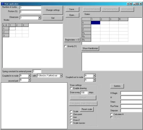
As mentioned before the program consists of two parts, the main application and the DLL. A screenshot of the main application is shown in Figure 13: Screenshot of main application (1).
Figure 13: Screenshot of main application (1)
The main application makes it possible to create a model and with this model a Hamiltonian which is used for the simulation. The main application uses nodes and stiffnesses to create a model. This is shown in the upper left table of the main application. With this matrix a model can be created and this model is used to create the Hamiltonian. The variables in the upper left corner are used to change the basics of the model, number of nodes, friction and dimension. The button ‘change settings’ is used to create the model and the Hamiltonian. When the program is started it is also able to read the
information from the shared memory if the shared memory exists with the button ‘Get’.
The buttons ‘Open…’ and ‘Save…’ are used to open and save a model. The button below ‘Beginstates -> D’ is used to calculate the distances for the stiffnesses in rest when the begin states are given. So when a node is created at location (0,0,0) and a second node at location (1,1,1) with a stiffness
Control Engineering
The upper right table shows the begin states and states when the buttons above are pressed. With the button ‘Set beginstates’ the beginstates of the model can be altered. The states of ‘R’ are the states of a zero mass node which has a spring connected to each node. This can be seen as a ‘bowl’ where the whole model is lying in. The stiffness of each node to this bowl is shown in ‘Spring constant for external power’.
Below the table of the states a textbox is shown to show the Hamiltonian when the ‘Show Hamiltonian’ button is pressed.
The lower left corner is used to draw the model. The Y-direction is vertical, the X-direction is horizontal and the Z-direction is in depth of the screen. On the right of the drawing the draw settings can be altered. The buttons ‘Default’, ‘Draw states’ and ‘Draw Beginstates’ are used to change the model which will be drawn. ‘Default’ draws only when simulating. ‘Draw states’ will draw the current states and ‘Draw Beginstates’ is used to draw the initial states. When the checkbox ‘Enable drawing’ is unchecked the viewthread is suspended and nothing is drawn. If checked the viewthread is resumed and the drawing will continue.
Above the drawing and below the matrix to change the model, the settings are shown for power coupling. The power is coupled to other 20-sim parts with two ports, each port is defined with an effort and a flow. The effort is the force and the flow is the velocity, as mentioned in chapter 2. The model has two ports. Each input is connected to a separate node or to the ‘bowl’, R. The R is a zero mass node which has a stiffness attached to each node. So when as force is applied on R all the nodes receive a force.
The way the inputs are used is shown in the pull down menu on the left. Two options can be chosen. The flow in and effort out or the effort in and flow out. The outputs are defined next to it. The outputs are also represented by a node or R.
So when effort in, flow out is selected the inputs are forces which acts on the nodes. The output is the velocity of the nodes when simulating. More information about the models can be found in the chapter 4.
University of Twente
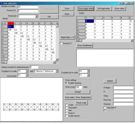
If the main application has a model loaded it will looks like Figure 14: Screenshot of main application (2).
Figure 14: Screenshot of main application (2)
Control Engineering
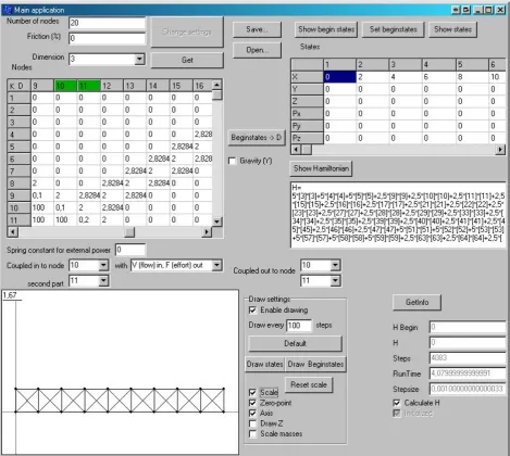
Figure 15: Screenshot of main application (3)
Control Engineering
4 Model
testing
To test the module and its functionality several models where tested to see if the whole idea worked. All models which where tested are described in this section.
4.1 Preferred
causality
This section is used to explain what kind of storage element the written module is, and how it can be used in a natural way.
As mentioned before the written module uses the port concept to transfer energy to and from the system. Each energy storage element has a preferred causality. For example, a mass is a p-type storage element, which has the integral of effort (force), i.e. momentum as preserved quantity. The p-type storage element uses the integral of flow (velocity) to define the equilibrium and the effort to adjust the equilibrium. The preferred causality is effort in and flow out. The q-type storage element has flow as preserved quantity, effort to define the equilibrium and flow to adjust the equilibrium. This
preferred causality is flow in and effort out. An example of a q-type storage element is a spring. More information about the port concept can be found in (Dynamical systems, 2003).
Each storage element is a p-type of q-type storage element, the preferred causality is the type of buffer the storage element wants to be. So a mass storage element prefers effort in and flow out because it is a p-type storage element. The module for 20-sim, which calculates the Hamiltonian models for 20-sim consists of springs and masses, because the springs are q-type storage elements and masses are p-type storage elements it is hard to determine if the module is a p-type or q-type storage element. Therefore some analyzing must be done to determine this.
Each Hamiltonian model consists of masses and stiffnesses. The masses are always at the end of the model. The energy, which is coupled to the model, is always attached to a node. For example if a simple model is taken with 3 masses and 2 springs, as shown in Figure 12. When energy is coupled to this system, it is applied on one of the masses. If the energy is applied on the most right mass, the other two masses will interact with the first mass which has the energy applied to it. Because the energy is always coupled to a mass the Hamiltonian acts as a p-type storage element, but there is an exception. If the energy is coupled to the R the energy is applied straight to a stiffness, to a spring. So when energy is applied on the R the module acts as a q-type storage element.
When the module is used as a q-type storage element it can be seen how a model responds when it is shaken. It is more natural to use the module as a p-type storage element. This is when a beam is modeled and the user wants to know how it will react when a force is applied on the beam. So the user can see how strong the beam is and when it starts to bend or fold.
University of Twente
4.2 Static
modelsl
4.2.1 Poisson’s ratio
This model is to test how the stiffnesses of a model influences the Poisson ratio. The Poisson ratio is the ratio between the contraction strain divided by the relative extension strain. So the ratio between of bar shortens by a force and the ticker it will become. This is shown in the picture below.
Figure 16: Poisson ratio example
The bar gets shorter and thicker when a uniform force is applied on the bar. The Poisson formula for a 3-dimensional bar is given by:
x
The model which is used to test the relation between the stiffnesses and the Poisson ratio is shown in Figure 17: The model for testing the Poisson's ratio.
Figure 17: The model for testing the Poisson's ratio
The model represents a beam. The two left nodes are fixed and the two right nodes have a fixed Y position, so they only can move horizontally. The model is a 2-dimensional model. Therefore the Poisson ratio formula shown above cannot be used. The strain in z-direction,
ε
z,is fixed to 0 when a 2-dimensional model is used. The Poisson ratio formula for a 2-dimensional situation is:1
The strain in the y-direction is bigger due to the fact that the strain in z-direction is fixed to zero. This formula is used to determine the Poisson ratio, v. More information about theory of plates and the 2-dimensional Poisson ratio can be found in (Theory of plates and shells, 1959).
Control Engineering
The first test is how the vertical stiffness influences the Poisson ratio. Results are shown in Table 2.
Table 2: Results when changing K vertical
The Y5 and Y6 column represents the Y value of point 5 and 6 and Y15 and Y16 the Y value of point 15 and 16. These are the four points in the middle of the model and they are used to determine the height of the model. The X10 and X11 represents the X value of the most right nodes, they are used to determine the length of the model.
Poisson ratios above 0.5 are not realistic, because these materials do not exist. Rubber has the highest Poisson ratio of 0.5 and cork the lowest of 0. Materials like metal have a Poisson ratio around 0.3 and concrete about 0.2. A Poisson ratio of 0 is hard to model because the stiffness is infinite in vertical direction, all other materials can be modeled.
There are also materials with a negative Poisson ratio. This means when a bar is compressed is gets thicker instead of thinner. These materials are known as auxetics and they cannot be modeled with the written module.
A graph of the Poisson ratio as function of K vertical is shown in Figure 18.
University of Twente
The model is also tested when changing K diagonally. All other stiffnesses remained 100Nm. These results are shown below.
Table 3: Results when changing K diagonal
Figure 19: Graph when changing K diagonal
In the second test the model became unstable when the stiffness in diagonal direction was smaller than 40Nm, the result of this simulation is shown in Figure 20. It can be seen that the beam is not as it should be, and therefore it is unstable. Then most right nodes starts to move further left than the second most right nodes. This is impossible with a normal beam, therefore it can be concluded that the model is unsuitable for this situation.
Figure 20: Unstable model
The model only has values for K which are useful and K’s which causes the Poisson ratio to be smaller than 0.5.
Control Engineering
4.2.2 Clamped beam with a force
When a beam is clamped and a force is applied on the beam the beam starts to bend. Bending of a beam is tested in two ways, the first situation is a single clamped beam and the second situation is a beam with both sides supported. The first situation is shown in the figure below.
Figure 21: Single clamped beam
The single clamped beam has a formula to calculate the deflection of a beam. This formula is taken from (Mechanics of materials, 2001).
This formula is: the beam, x the position of deflection and EI the material constant. This formula applies only for small deflections.
So when a model is made with the written module, the EI variable must remain constant at every position of the beam even when the force is changed. The model used is shown in Figure 22: Single clamped beam.
Figure 22: Single clamped beam model
The model has the two left nodes clamped. A force is pressing on the top-right node. Each stiffness is 200Nm and each point mass is 0.2kg, the length between the nodes is 2m. So when a force is applied the beam should bend. The total deflection is depended of the force, so for each force and each position the same material constant EI must be obtained. EI is defined as
(
)
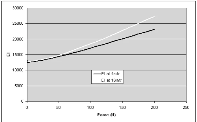
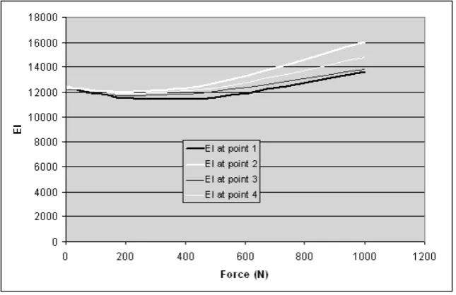
University of Twente Table 4: Results from first measurement
The comparison of EI at 4 meter and EI at 16 meter is shown below.
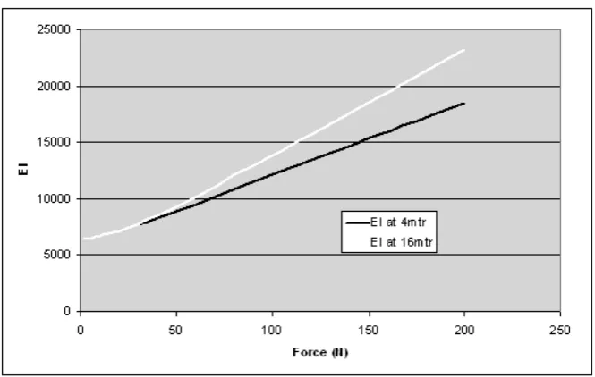
Figure 23: Graph of EI at 4 meter and at 16 meter
The EI should be constant for each force and at both positions. The results should be a horizontal line instead of a curve. When the force is rather small, less than 40N, the model is sufficient because it does not differ a lot from the results obtained by the formula. If the force gets larger this formula is not sufficient enough and the results differ a lot.
Control Engineering
In the next plot the difference in terms of percentage between EI at 4m is compared to the EI at 16m.
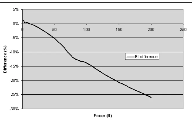
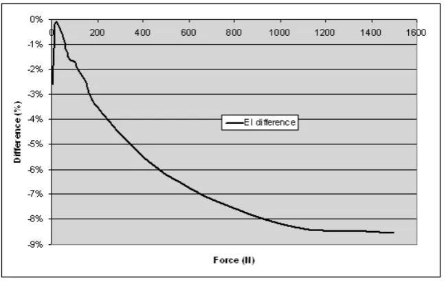
Figure 24: EI difference between 4m and 16m
In this graph it clearly can be seen that the formula is sufficient for small forces, less than 40N, because the difference between EI is less than 5%. There are two common reasons why the EI
difference in terms of percentage increases while the force increases. The most likely reason for this is that the formula used to calculate the EI constant only works for small deflections, when the
deflections are too big the formula cannot be used which results in incorrect results. The second reason is that the model is not good enough to represent a beam. The model only uses point masses and stiffnesses. And a real beam has more aspects than point masses and stiffnesses.
In Figure 25 the model is shown after 60seconds when 200N of force is applied. It can be seen that the beam has a large deflection, therefore the formula from (Mechanics of materials, 2001) is not
sufficient enough for this kind model with 200N of force.
Figure 25: Single clamped beam with 200N of force
The bending mostly occurs in the beginning of the beam. At the end the beam is more stretched than bended. Therefore the beam looks stronger at the end than at the beginning. A beam is stronger when stretched than bended. This explains the large differences of the EI constant between the point at 4m and at 16m, shown in Figure 24.
University of Twente Table 5: Results from second measurement
A graph of the EI difference between 4m and 16m is shown below.
Figure 26: Graph of EI difference between 4 and 16 meter from second measurement
Control Engineering
The difference in terms of percentage is also plotted, shown below.
Figure 27: EI difference at 4m compared to EI at 16m from second measurement
This graph shows also that the linear formula is sufficient for a small force, less than 40N. When this force gets larger the differences of the EI constants become larger. This happens because the beam bends in the beginning and is only stretched at the end.
At the end the difference in terms of percentage is larger because the beam is weaker than the beam used in the first measurement, so the difference is also greater.
The conclusion for this test is that the model is not sufficient to model a beam, because the EI constant is not the same at each point of the beam and the EI constant changes when the force changes. The linear formula is sufficient when small forces are used but for larger forces the formula is not
sufficient enough. For small deflections the EI should be constant using the deflection formula, this is not the case, therefore the model is not sufficient enough. When a weaker beam is modeled the differences between EI become even larger with large forces. With a stiffer beam these differences are not that large. So the model works for stiff, strong beams with a small force. The difference of the EI constant between the beginning of the beam and the end is caused by a large force. The bend point is in the beginning of the beam, the end is therefore more stretched than bended and this causes the EI constant to become smaller at the beginning of the beam than at the end of the beam, this effect cannot be described with the deflection formula.
University of Twente
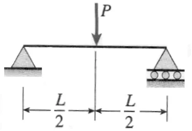
4.2.3 Dual supported beam
Secondly a model is tested with both sides supported. One side is supported and the other side can only move in horizontal direction. A figure of this situation is shown below.
Figure 28: Dual supported beam
It can be seen that the left side can move horizontally. The model is carried on the bottom right node and the bottom left node. The model which is used is the same as the test with a single clamped beam, shown in Figure 22: Single clamped beam model.
The deflection for this situation can be calculated with:
(
2 2)
the beam, x the position of the deflection and EI the material constant. The formula only works for small deflections. This formula can be rewritten to calculate the material constant, EI, to(
2 2)
With this formula the EI is calculated at several points of the beam. The figure below shows the points where EI is calculated.
Figure 29: Points where EI is calculated
Control Engineering
Table 6: Dual clamped beam results (1)
The graph of these results are shown below.
Figure 30: Graph of first results
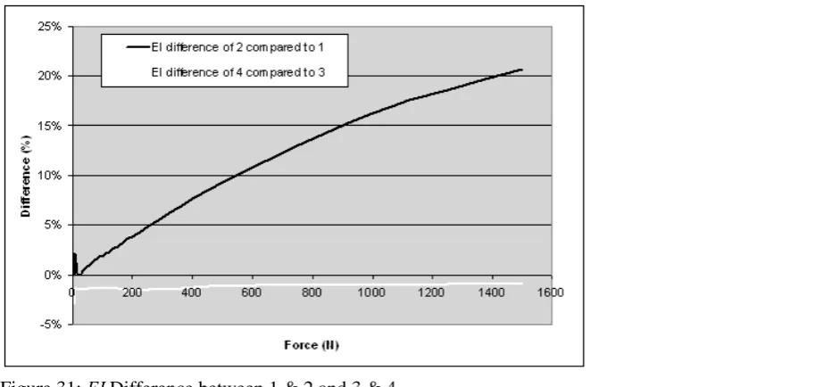
Second the EI differences between point 2 compared to point 1 and point 3 compared to point 4 are plotted. The difference between these values should be zero.
University of Twente
The difference of EI between point 4 and 3 is minimal, therefore the force is not deforming the beam much in vertical direction. The difference of EI between point 1 and point 2 gets larger while the force gets larger. This happens because point 1 and point 2 do not only down but they also rotate around the most left point, where the beam is supported. This is shown in Figure 33. The difference is caused by this rotation.
Next the EI difference between point 1 and point 3 is plotted.
Figure 32: EI difference between point 1 and 3
The EI difference between point 1 and point 3 gets larger when the force gets larger. This is the same as what happened to the single clamped beam. The model is also stronger when it is stretched than bended, therefore the EI constant is larger at point 3 than at point 1. The bending happens mostly at point 1, point 3 is not bended that much. This is shown below.
Figure 33: dual clamped beam with 1500N force
Control Engineering
This model is also tested with the force applied to point 3 instead point 4. These results are shown below.
Table 7: Dual supported beam results (2)
The graph of the second measurement results is shown below.
Figure 34: Results of second measurement
University of Twente
Next the EI difference between point 2 and point 1 and the difference between point 4 and point 3 is plotted. This is shown below.
Figure 35: EI Difference between 1 & 2 and 3 & 4 for second measurement
The difference between point 4 and point 3 is increasing because the force is not applied on point 4 but on point 3. Therefore the EI difference between those points gets larger compared to the first
measurement. The difference between point 2 and point 1 looks the same compared to the first measurement. This difference has also the same explanation.
The difference between point 1 and point 3 is also drawn.
Figure 36 EI difference between point 1 and 3 for second measurement
This figure shows that the EI difference gets larger when the force gets larger. After 500N the
difference decreases again. This happens because the force is applies on point 3 instead of point 4. The first part is the same as the first measurement. Because the force is applies on point 3 is pushed further down than in the first measurement. When point 3 is pushed further down the calculated EI will become smaller, therefore the difference become smaller after 500N. With a force less than 500N this difference cannot be seen because the beam is stiff enough to compensate this.
Control Engineering
4.3 Dynamic
models
4.3.1 Mass on a spring
The first dynamic model is a simple mass on a spring, shown in the picture below.
Figure 37: Mass on a spring
The model has gravity enabled and the spring is in rest. So when the simulation starts the mass must start to resonate and at the end it stops resonating with the spring stretched out.
The results are shown in the graph below.
Figure 38: Results of mass-spring
The main application shows that the spring is stretched by 0.189m. To see if the results are correct the model can be calculated.
The force on the mass is
9.81*10 98.1
F =ma= =
The force on the spring is defined as
2 2 2
2 (
)
200(
1)
F
=
k x
−
d x
=
x
−
x
So the stand at ease is
2
100(
1)
98.1
1.89
x
x
x
−
=
=
University of Twente Figure 39: Graph of 4th order spring energy, d=1
The plot has horizontal the length of the spring, with 1 as rest length. The ‘spring constant’ k is
100Nm. The function plotted therefore is
1
(
2 2)
250
(
21
)
22
V
=
k l
−
d
=
l
−
. This clearly shows energyis needed to push the spring in. Because the energy function is a 4th order function, the function changes a lot which results in a much higher ‘spring constant’. This is shown in the plot below where
the d is increased to 2 and the function become:
V
=
50
(
l
2−
4
)
2Figure 40: Graph of 4th order spring energy, d=2
Control Engineering
Figure 41: results when d is 2
The spring is lengthened by 0.059m and therefore the actual spring constant is much higher.
This can be shown with the following equation
1
(
2 2)
21
(
)
2(
)
22
2
V
=
k l
−
d
=
k l d
+
l d
−
. The actualUniversity of Twente
4.3.2 Mass on a chain
The next model which is tested is a mass on a chain. The chain consists of 11 nodes, the space between each node is 2m. Each node has a mass of 0.2kg and at the end a mass of 10kg is mounted. The chain gets a momentum by a force of 1000N which is applied to the left side for 0.3seconds at the end mass. The model of the beam is shown below. The top node is located at the location (x,y) (0,22) and is fixed. The model is simulated with the Euler integration method with a step size of 0.001 second.
Figure 42: Begin state of mass of a chain
Due to the gravity force the chain will extend a little, this rest position is the begin position when the force is applied. The chain is lengthened by 0.33m, so the total length will be 20.33m.
After the momentum was applied on the beam the states of the bottom mass, kinetic and potential energy where measured at a several time intervals. A lot of results were obtained, because there are many results, these are shown in appendix I.
First the path of the moving mass is plotted. This is shown below.
Control Engineering
The thick white line is a reference path. This reference path is part of a circle with a center at (0,22) with a radius of 20.33.
The thin black line is the first half swing, from bottom to top. The measurement is started right after the force has stopped. The mass gets of course between x is -5 and 15. This happens because the force is applied in x-direction. The momentum causes the chain to stretch a bit and starts to resonate in axial direction. After a while it will shorten due to the stiffnesses in the chain. This result is shown between x is 15 and 18. A picture was also taken at this part. This picture was taken after 1.475 seconds of simulation and is shown below.
Figure 44: Chained mass during simulation
This picture shows that the chain is shortened due to momentum it was given at the beginning. The chain in this figure does not have the same kinetic energy as the end mass and it is a little slower than the end mass, therefore the chain is curved.
The second swing, from far left to far right, starts with a slightly shortened chain due to the first swing. Some resonating can be seen in axial direction around x is 18 and x is 14. At x is 0 it can be seen that the chain is a bit longer than the reference path. This happened due to the centrifugal force. The kinetic energy of the mass causes the chain to stretch at x is 0. When the energy is decreased the reference path is followed correctly.
The forth swing has so less energy that the chain will not deform anymore and the reference path is followed precisely. The forth swing stops at x is 0 and is slightly thicker than the third swing.
Next the radius of the chain is plotted during simulation. This is shown in Figure 45.
Figure 45: Radius of chain
University of Twente
After 8 seconds the major resonation has stopped. The little vibrations after 8seconds are caused by a resonating between the nodes themselves which has not been damped by friction yet.
To determine the period of the swing the angle over time is plotted.
Figure 46: Angle over time
With this figure the swing period can be determined. The swing period is the period from the
minimum at 2.6seconds and the minimum at 12.3seconds. This period is 9.7seconds. This period can also be determined by plotting the kinetic energy over time. This is shown below.
Figure 47: Kinetic energy over time
The period of a swing is the time between the first zero point and the third. These are located at 2.6seconds and 12.3seconds. This also gives a period of 9.7seconds. Both graphs gave the same result, as they should be. The second graph is only to check if this is the case.
Control Engineering
Fig