A Quantitative Prediction Method for Fracture

(1)

A Quantitative Prediction Method for Fracture

1 Density Based on the Equivalent Medium Theory

2

Liang Sun 1,2_{, Suping Peng}1,2_{*, Dengke He}1,2_{, Shu Wang}1,2

3

1_{State Key Laboratory of Coal Resources and Safe Mining, China University of Mining and Technology}

4

(Beijing), Haidian, Beijing 100083, China; [email protected] (L.S.); [email protected] (D.H.);

5

[email protected] (S.W.)

6

2 _{College of Geoscience and Surveying Engineering, China University of Mining and Technology (Beijing),}

7

Haidian, Beijing 100083, China

8

* Correspondence: [email protected]

9

10

Abstract: Fracture density, a critical parameter of unconventional reservoirs, can be used to evaluate

11

potential of unconventional reservoirs and location of production wells. Many technologies, such

12

as amplitude variation with offset and azimuth (AVOA) technology, vertical seismic profiling (VSP)

13

technology, and multicomponent seismic technology, are generally used to predict fracture of

14

reservoirs. they can qualitatively predict fractureby analyzing seismic attributes, including seismic

15

wave amplitudes, seismic wave velocities, which are sensitive to fracture. However, it is important

16

to quantitatively describe fracture of reservoirs. In this study, based on a double-layer model, the

17

relationships between fracture density and the double-layer model’s physical parameters, such as

18

velocity of fast shear-wave, velocity of slow shear-wave, and density, were established, and then a

19

powerful quantitative prediction method for fracture density was proposed dramatically.

20

Afterwards, the Hudson model for crack was used to test the applicability of the method. The result

21

shown that the quantitative prediction method for fracture density can be applied suitable to the

22

Hudson model for crack. Finally, the result of validation models indicated that the method can

23

predict fracture density effective, in which absolute relative deviation (ARD) were less than 5% and

24

root-mean-square error (RMSE) was 4.88×10-3_.

25

Keywords: Fracture density; Double-layer model; Unconventional reservoirs; Multicomponent

26

seismic; Shear-wave splitting

27

28

1. Introduction

29

Unconventional resources have received widespread interest in recent years because of their

30

emergence as a source of clean energy, and they are now being developed and produced in North

31

American shales, Southern North China shales, etc. [1-3]. As self-sourced reservoirs, the fracture

32

space controls not only the potential of unconventional reservoirs but also location of production

33

wells [4]. Thus, the accurate prediction of fracture density plays an important role in the exploration

34

and development of unconventional reservoirs. In particular, knowing the fracture density variation

35

between zones within a reservoir can help in the accurate determination of well locations [5].

36

Many achievements have been made with the continuous improvements by researchers for

37

predicting the fracture in sedimentary strata [6-9]. Sedimentary strata, such as unconventional

38

reservoirs, are usually described as anisotropic mediums on the scale of seismic waves, and the

39

anisotropy of a medium is produced by skeleton orientated arrangement and fracture development

40

[10-11]. Ruger (1997, 2002) researched the relationship among P-wave reflection coefficients, offset,

41

and azimuth named AVOA technology, which was found to be suitable for analyzing the anisotropy

42

of a medium [12-13]. While, some researchers used the AVOA technology to predict the anisotropy

43

of fractured reservoirs for analyzing the fracture development, and the results in these studies were

44

presented by anisotropic parameters to reflect the fracture development [9, 13-15]. Thus, the AVOA

45

technology was a non-direct way to predict the fracture development of reservoirs clearly.

46

(2)

Using the vertical seismic profiling (VSP) technology to predict the fracture development of

47

reservoirs is realized by the splitting property of the S-wave, the S-wave split into fast S-wave and

48

slow S-wave when passing through fracture with an angle[16-17], which is obviously different from

49

AVOA technology. The difference between the velocities of these waves can be estimated by

50

measuring the increase of the time delay between them with the depth [18]. Meadows et al. [19],

51

Pevzner et al. [20], and Shevchenko et al. [21] used VSP technology to predict the fracture of

52

reservoirs. The prediction results shown that the VSP technology can estimate the S-wave anisotropy

53

of reservoirs by the difference between the fast S-wave velocity and the slow S-wave velocity, which

54

was useful for representing the fracture development of reservoirs. However, this technology

55

requires a borehole that is available for the exploration area. Thus, it only has the ability to reflect

56

the fracture development near the borehole, actually. Ata et al. [22], Gaiser [23] and Vetri et al. [24]

57

used multicomponent seismic technology to predict the fracture development of reservoirs by

S-58

wave splitting property. Compare with the VSP technology, multicomponent seismic data did not

59

have the advantage of recording data near the reservoirs, which can bypass complications introduced

60

by the overburden. Fortunately, with the improvement of multicomponent seismic data acquisition

61

and processing technology [25-31], the application of multicomponent seismic technology has

62

gradually increased, providing favorable technical support for identifying the fracture of reservoirs

63

[32-33]. However, Using the splitting property of the S-wave to predict the fracture of reservoirs is

64

also a non-direct way yet.

65

During the past few decades, the equivalent medium theory, a method for digitizing rocks, has

66

attracted the attention of many researchers [34-36]. Backus [37] demonstrated that a multilayer

67

transversely isotropic medium was equivalent anisotropic if the wavelength of seismic wave is much

68

larger than the monolayer of the multilayer transversely isotropic medium, and then the equivalent

69

elastic tensor of this medium was given. Eshelby [38] studied the situation of a single elliptical

70

inclusion in isotropic media, and then Cheng [39] gave the equivalent elastic tensor of the situation.

71

Hudson [40] researched the condition that fracture is represented as a gap or inclusion with a thin

72

coin-shaped ellipsoid, and provided the equivalent elastic tensor. Schoenberg [41] ignored the shape

73

and microstructure of fracture and considered the fracture was an infinitely thin and very soft

74

stratum satisfying the linear sliding boundary condition. While, a linear sliding model was proposed.

75

Subsequently, the equivalent medium theory has been developed and promoted [42-46].

76

Based on the equivalent medium theory, this study established the relationships among fracture

77

density, multicomponent seismic response, density. As a result, a powerful quantitative prediction

78

method for fracture density was proposed. Furthermore, the applicability of the quantitative

79

prediction method for fracture density was verified by the Hudson model for crack. In this study,

80

Section 2 addresses details to construct a quantitative prediction method for fracture density based

81

on an equivalent medium model. Section 3 verifies the quantitative prediction method for fracture

82

density with the Hudson model for crack. The data to test the proposed method and discussion in

83

this study are presented in Section 4. Finally, conclusions are presented in Section 5.

84

2. Method Assumptions and Establishment

85

In this section, firstly, we make some idealized assumptions in order to achieve a powerful

86

method for predicting fracture density. Secondly, the relationships between the fracture density and

87

the physical parameters of target layer, such as fast S-wave velocity, slow S-wave velocity, root mean

88

square (RMS) velocity, and density, are developed under the idealized assumptions. Finally,

89

calculation Eqs. for the fracture density are given in detail, and then a quantitative prediction method

90

for fracture density is established.

91

2.1 Assumptions

92

As a result of their genesis, sedimentary strata, such as unconventional reservoirs, can be

93

exhibited in a thin interbedded medium. In this work, we assume that the thin interbedded medium,

94

shown in Fig. 1, is composed of two components: rock skeleton layer (matrix) represented by black

95

(3)

Moreover, following assumptions and simplifications are made to generate a practical method for

97

predicting the fracture density which is defined by the volumetric proportion between the fracture

98

layer and the total layer.

99

100

Figure 1. Thin interbedded medium

101

(1) The rock layer and rock fracture layer of the thin interbedded medium are assumed isotropic,

102

homogeneous, and linear elastic.

103

(2) There are no sources of intrinsic energy dissipation, such as friction or viscosity, between

104

the rock skeleton layer and the rock fracture layer.

105

(3) The thickness of the rock skeleton layer and the rock fracture layer must be much smaller

106

than a seismic wavelength, which the seismic wavelength must be at least ten times a layer

107

thickness.

108

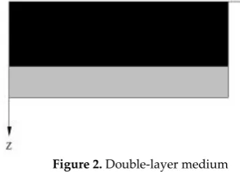
According to the aforementioned assumptions, we can divide the thin interbedded medium into

109

two parts: a skeleton layer and a fracture layer, and then the thin interbedded medium can be

110

equivalent to a double-layer medium. Fig. 2 shows the double-layer medium, in which the black part

111

represents the skeleton layer and the gray part indicates the fracture layer.

112

113

Figure 2. Double-layer medium

114

2.2 The relationships between S-wave velocities and fracture density

115

Notable, Backus (1962) demonstrated that if the wavelength of seismic wave is much larger than

116

the monolayer of the thin interbedded medium, it will be equivalent anisotropic [37]. Thus, the

117

stiffness tensor (

C

) of the double-layer medium can be represented facile by Backus Average, which

118

depicted with the P-wave velocity (

V

_P), the S-wave velocity (

V

S), the density (



), and the volume

119

of each layer.

120

Table 1 Physical parameters of the double-layer medium

121

P-wave velocity (m/s) S-wave velocity (m/s) Density (kg/m3₎ _{Volume (m}3₎

Skeleton layer VP1 VS1  d1

Fracture layer VP2 VS1  d2

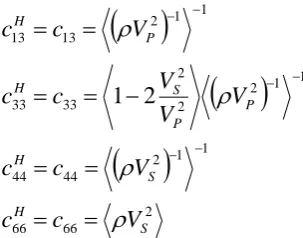
Tab. 1 shows the physical parameters of the double-layer medium, and then the stiffness tensor

122

(

C

) of the double-layer medium can be described through Backus average [37] and Levin formula

123

(4)

11 12 13

12 11 13

13 13 33

44

55

66

0

0 c

c

C

c

















 























(1)

125

where

c

₅₅



c

₄₄

;

c

66



0.5 

c

11



c

12



;

126

2

2 2

1

2 2 1

11 2 2

2

2 2

1

2 2 1

12 2 2

2 2

1 2 1

13 2

1 2 1 33

1 2 1 44

2 66

4

1 1 2

(

)

2 1 2

1 2

(

)

1 2

(

)

(

)

(

)

S S

S P

P P

S S

S P

P P

S

P P

P S S

V

c

V

c

V

c

V

c

V

c

V

c

V



 



_

_





_



_

 

















_



_

 











_{ }



_



_



_



127

The brackets



indicates averages of the enclosed properties weighted by their volumetric

128

proportions, which is often called the Backus average. As a result, we can represent the fast S-wave

129

velocity (

V

_Fast) and the slow S-wave velocity (

V

_Slow) of the double-layer medium as follows:

130

2 2

66

(

1 1 1 2 2 2

) (

1 1 2 2

)

Fast all S S

V



c





f



V



f



V

f





f



(2)

131

2 2 1

44

(

1 1 1 2 2 2

)

(

1 1 2 2

)

Slow all S S

V



c





f



V



f



V



f





f



(3)

132

where



_all



f

₁



₁



f

₂



₂ denotes the average density, kg/m3_;

1

1 f

 



represents the

133

volumetric proportion between the skeleton layer and the total layer with the range (0, 1],

134

dimensionless;

f

₂





indicatesthe volumetric proportion between the fracture layer and the total

135

layer with the range [0, 1), dimensionless;





d

2



d

1



d

2



is the fracture density with the range

136

[0, 1), dimensionless.

137

2.3 The relationships between root mean square (RMS) velocities and fracture density

138

On the basis of above-mentioned, we can develop the relationships between root mean square

139

(RMS) velocities and the fracture density. In this study, the P-wave RMS velocity (

V

_P) in the

double-140

layer medium can be expressed as:

141

2 1

2 2 2 2

1 1

t

V

t

V

t

V

P P

P

_



(5)

where

t

1



d V

1 P1 represents the vertical propagation time of P-wave in the skeleton layer, s;

143

2 2 P2

t



d V

denotesthe vertical propagation time of P-wave in the fracture layer, s. Moreover, the

144

physical parameters of the skeleton layer and the fracture layer, shown in Table 1, are substituted

145

into Eq. (4), we can obtain:

146

2 2

1 1

2 2 2 2 2

1 1 1

P P

P P P P P

V

d

V

d

V

d

V

d

V





(5)

147

Through further simplification, the Eq. (5) can be rewritten:

148 







11 22

1

P P

P

P P

V













(6)

149

In the same way, the S-wave RMS velocity (

V

S) can be obtained as follows:

150 







11 22

1

S S S

S S

V













(7)

151

2.4 The relationship between P-wave velocity and density

152

Gardner [48] and Castagna [49] studied the relationship between the P-wave velocity and the

153

density in different lithology, and then determined their relationships. Gardner [48] suggested an

154

empirical relation between the P-wave velocity (

V

_G) and the density (



G) that represents an average

155

over many rock types:

156

25 . 0

741 .

1

_G

G



V



(8)

157

where

V

_G is in km/s and



G is in g/cm3, or

158

25 . 0

23 .

0

_G

G



V



(9)

159

where

V

_G is in ft/s.

160

2.5 The quantitative prediction method of fracture density

161

Through aforementioned Eqs. on the relationships between the fracture density and the physical

162

parameters of the double-layer medium, such as the fast S-wave velocity, the slow S-wave velocity,

163

the root mean square (RMS) velocity, and the density, the key issue required to be solved is how to

164

establish a practical method for predicting fracture density.

165

After the analysis on the correlations of the Eqs. above, we consider to build the relationship

166

between the P-wave velocity and density of a target layer firstly, which is according to the studies by

167

Gardner [48] and Castagna [49]. Actually speaking, a certain amount of core analysis and logging

168

data will be finished before development of an unconventional reservoir, and as a result the

non-169

linear relationships between the P-wave velocity and the density of the target layer can be obtained:

170

25 . 0

1 1



aV

P



(10)

171

25 . 0 2 2



bV

P



(11)

(6)

where coefficient a reflects the relationship between the P-wave velocity and the density of the

173

skeleton layer, dimensionless; coefficient b indicates the relationship between the P-wave velocity

174

and the density of the fracture layer, dimensionless. Meanwhile, the average density (



_all) of the

175

target layer can also be obtained:

176

2 2 1

1



_all



f



f

(12)

177

Furthermore, taking Eq. (10) and Eq. (11) into Eq. (6), and its expression Eq. was as follows:

178 







4 4

1 2

4 4

1 2

1 1 (

)

(

)

1 1 (

)

1 (

)

P

a

b

V

a

b



















(13)

179

Notable, the RMS velocities about the P-wave and wave, and the velocities about the fast

S-180

wave and the slow S-wave of the prospecting stratum are acquired from a conventional data

181

processing of multicomponent seismic exploration. Moreover, the average density can be obtained

182

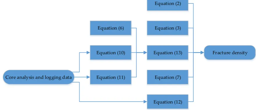
from the core analysis and logging data of survey area. Finally, the fracture density can be achieved

183

through solving the Eq. (2), Eq. (3), Eq. (7), Eq. (12), and Eq. (13), and the flowchart of the calculation

184

is illustrated in Fig. 3. According to the aforementioned analysis, we established the quantitative

185

prediction method of fracture density for the first time in this way.

186

Equation (2)

Equation (3)

Equation (13)

Equation (7)

Equation (12) Core analysis and logging data

Equation (10) Equation (6)

Equation (11)

Fracture density

187

Figure 3 Flowchart of the calculation

188

3. Application in Hudson Model for Crack

189

3.1 The quantitative prediction method of fracture density application analysis in Hudson Model for crack

190

The quantitative method above assumed that a sedimentary stratum consisted of a layered

191

skeleton and a layered fracture. However, fractured strata are often depictedwith the Hudson model

192

in seismic prospecting [40], in whichthe fracture is represented as a gap or inclusion with a thin

coin-193

shaped ellipsoid. It is feasible to predict the fracture density about the Hudson model by the new

194

method if the velocities about the fast S-wave and slow S-wave are acquired from the seismic data

195

processing and the RMS velocities about the P-wave and S-wave can be converted by some skills.

196

Actually speaking, the velocity group consisted of the four velocities above is just the seismic

197

responses about the given model, including the Hudson model and the other equivalent models,

198

which is the concrete links for predicting the fracture density about the Hudson model by the new

199

method based on the double-layer model. The stiffness tensor is the essential factor for the seismic

200

responses. Therefore, the new method can predict the fracture density of the Hudson model if the

201

parameters about the double-layer model can be determined by the stiffness tensor of the Hudson

202

model according to the Eq. (1), which can deduce the RMS velocities about the P-wave and S-wave.

203

The key for applying and verifying the new method to the Hudson model is how to represent the Eq.

204

(7)

the velocities about the double-layer model by the Hudson model parameters according to the Eq.

206

(1).

207

208

Figure 4. Hudson model for crack

209

Fig. 4 represents the Hudson model, in which black denotes the skeleton part and gray indicates

210

the fracture part. The physical parameters of the Hudson model are shown in Tab. 2, includingthe

211

P-wave velocity, the S-wave velocity, the density, and the volume of each part, which can depict the

212

stiffness tensor of the Hudson model at any crack width ratio (



H ). Meanwhile, the fracture density

213

(



) is also defined by the volumetric proportion between the fracture part and the total part.

214

Table 2 Physical parameters of the Hudson model for crack

215

P-wave velocity (m/s) S-wave velocity (m/s) Density (kg/m3₎ _{Volume (m}3₎

Skeleton part 1

H P

V

H₁

S

V



₁H_

1

H

d

Fracture part 2

H P

V

2

H S

V

2

H



2

H

d

According to above analysis, we consider that the



₁,



₂, and



of the double-layer model

216

are equal to



₁H ,



₂H , and



H of the Hudson model, respectively. By adjusting the

V

_P₁,

V

_S₁,

217

2

P

V

, and

V

_S₂ to make the stiffness tensor of the double-layer model equals to the stiffness tensor of

218

the Hudson model, and then the equivalent RMS velocities about the P-wave and S-wave of the

219

Hudson model can be obtained, which is the key for applying and verifying the new method to the

220

Hudson model. As a result, the above issue is converted to another form that is whether an unique

221

solution set of the

V

P1,

V

S1,

V

P2, and

V

S2 is existence to make the stiffness tensor of the

double-222

layer model equal to the stiffness tensor of the Hudson model.

223

3.2 Unique solution set determination

224

In order to obtain the unique solution set of the

V

_P₁,

V

_S₁,

V

_P₂, and

V

_S₂, the components of

225

the stiffness tensor (

c

13,

c

33,

c

44,

c

66) of the double-layer model are used to represent the

226

components of the stiffness tensor (

c

13H,

H

c

₃₃,

c

₄₄H ,

c

66H) of the Hudson model, respectively, which is

227

as follows:

228

 

2 66

66

1 1 2 44

44

1 1 2 2

2

33 33

1 1 2 13

13

2

1

S H

P P

S H

P H

V

c

V

c

V

c

V

c









 

  



(14)

229

(8)

2 2 2 2 2 1 1 1 66 2 2 2 2 2 1 1 1 44 2 2 2 2 2 2 1 2 1 1 33 13 2 2 2 2 2 1 1 1 13

1 )

2

1 (

)

2

1 (

1

S S H S S H P S P S H H P P H

V

f

V

f

c

V

f

V

f

c

V

f

V

f

c

V

f

V

f

c























(15)

231

For further simplification, we have defined some intermediate variables shown in Eqs. (17), and

232

then Eqs. (15) can be rewritten:

233

2 2 1 1 4 2 2 1 1 3 2 2 2 1 1 1 2 2 2 1 1 1

2

1 S

b

S

b

y

S

a

S

a

y

P

S

f

P

S

f

y

P

a

P

a

y

















(16)

234

where

235

H

c

y

13 1

1 

, _H

H

c

y

33 13

2



, H

c

y

44 3

1 

,

y

4



c

66H

236

1 1 1



f

a



,

2 2

2



f

a



,

b

₁



f

₁



₁ ,

b

₂



f

₂



₂ (17)

237

2 1 1

1

P

V

P



, ₂

2 2

1

P

V

P



,

S

1



V

S21,

2 2

2

V

S



238

There are two sets of solutions about the variables including the

S

1,

S

2,

P

1, and

P

2 which

239

has a certain relation with the

V

P1

,

V

S1

,

V

P2

,

and

V

S2, respectively, through solving the Eqs. (16),

240

and its expressions are as follows:

241 



2 2 2 2 2 2 1 2

4 1 1 2 2 3 4 1 1 1 2 1 2 1 1 3 4 2 2 2 2 3 4 3 4

3 1'

1

2 2 2 2 2 2 1 2

2 2 1 1 3 4 1 1 1 2 1 2 1 1 3 4 2 2 2 2 3 4 3 4

2'

2 3

2 2 2 2 2' 1

1'

2 1 1' 1 2 2'

1 (

(

2

2 ) )

2 (

2

2 )

2

2 y

a b

y y

a b

a a b b

a b y y

a b

a b y y

y y

y

S

b

a b

y y

a b

a a b b

a b y y

a b

a b y y

y y

S

b y

a y

a

f S y

P

a f S

P



























 

 







1 2 1 1 1' 1

2'

2 1 1' 1 2 2'

2

(9)





2 2 2 2 2 2 1 2

4 1 1 2 2 3 4 1 1 1 2 1 2 1 1 3 4 2 2 2 2 3 4 3 4

3 1*

1

2 2 2 2 2 2 1 2

2 2 1 1 3 4 1 1 1 2 1 2 1 1 3 4 2 2 2 2 3 4 3 4

2*

2 3

2 2 2 2 2* 1

1*

2 1 1* 1 2 2*

1 (

(

2

2 ) )

2 (

2

2 )

2

2 y

a b

y y

a b

a a b b

a b y y

a b

a b y y

y y

y

S

b

a b

y y

a b

a a b b

a b y y

a b

a b y y

y y

S

b y

a y

a

f S y

P

a f S

P































 

 





1 2 1 1 1* 1



2*

2 1 1* 1 2 2*

2

2 a y

a

f S y

a f S











_{ }









244

(19)

245

where apostrophe denotes the first set of solutions; asterisk represents the other set of solutions.

246

Substituting Eqs. (17) into Eqs. (18) and Eqs. (19), we can obtain:

247

2 2 66 66 2 2 2 66 2 2 2 1 2

66 44 2 1 1 2 1 2

2 44 44 44

1'

1 1

2 2 66 66 2 2 2 66 2 2 2 1 2

44 2 1 1 2 1 2

2 44 44 44

2'

2 2

2 1 2 1' 2 1 2 2' 1

1' 2

1 (

((

)

2(

)

(

) ) )

2

1 (

((

)

2(

)

(

) ) )

2 2(

)

H H H

H H

H H H

S

H H H

H

H H H

S

S S

P

c

f

c

V

f

c

f

c

V

f

f f V

V

f





























 

₂

13 2 33 2 2 2 2' 33

2 2

2 1 2 1' 2 1 2 2' 1

2' 2

1 13 1 33 1 1 1 1' 33

2 2(

)

2

H H H

S

S S

P H H H

S

c

f

f V

c

f f V

V

f c

c

f

f V

c



















_











(20)

248

2 2 66 66 2 2 2 66 2 2 2 1 2

66 44 1 2 1 2 1 2

2 44 44 44

1*

1 1

2 2 66 66 2 2 2 66 2 2 2 1 2

44 1 2 1 2 1 2

2 44 44 44

2*

2 2

2 1 2 1* 2 1 2 2* 1

1*

1 (

((

)

2(

)

(

) ) )

2

1 (

((

)

2(

)

(

) ) )

2 2(

)

H H H

H H

H H H

S

H H H

H

H H H

S

S S

P

c

f

c

V

f

c

f

c

V

f

f f V

V

f































 

₂

2 13 2 33 2 2 2 2* 33

2 2

2 1 2 1* 2 1 2 2* 1

2* 2

1 13 1 33 1 1 1 1* 33

2 2(

)

2

H H H

S

S S

P H H H

S

c

f

f V

c

f f V

V

f c

c

f

f V

c













_

_



_











(21)

249

According to the Appendix A, Eqs. (20) is not the reasonable solution for the

V

_S2₁,

V

_S2₂,

V

_P2₁,

250

and

V

_P2₂ under the requirement that the S-wave velocity of the skeleton part (

V

S21) should be larger

251

than the S-wave velocity of the fracture part (

V

S22) in the actual situation. Hence, the Eqs. (21) is the

(10)

only solution for the

V

S21, 2

2

S

V

,

V

P21, and

2 2

P

V

. Moreover, it is obviously that there will be have 16

253

sets of solutions for the

V

_S₁,

V

_S₂,

V

_P₁, and

V

_P₂, due to the four parameters at the left of the Eqs.

254

(21) are quadratic. Finally, the Eqs. (22) is the only solution about the Eqs. (21) with the positive

255

number, owing to the other solutions are eliminated under the actual situation that the seismic wave

256

velocities （

V

_S₁,

V

_S₂,

V

_P₁,

V

_P₂）must be real numbers larger than zero, which is as follows:

257

2 2 66 66 2 2 2 66 2 2 2 1 2

66 44 1 2 1 2 1 2

44 44 44

1*

1 1

2 2 66 66 2 2 2 66 2 2 2 1 2

44 1 2 1 2 1 2

44 44 44

2*

2 2

1 2 1* 2 1 2 2* 1

1*

2 1

1 (

((

)

2(

)

(

) ) )

2

1 (

((

)

2(

)

(

) ) )

2 2(

)

H H H

H H

H H H

S

H H H

H

H H H

S

S S

P

c

f

c

V

f

c

f

c

V

f

f f V

V

f c































 

₂

3 2 33 2 2 2 2* 33

2 2

1 2 1* 2 1 2 2* 1

2* 2

1 13 1 33 1 1 1 1* 33

2 2(

)

2

H H H

S

S S

P H H H

S

c

f

f V

c

f f V

V

f c

c

f

f V

c





















_



_

_



(22)

258

Based on the above analysis, there is a set of the P-wave and the S-wave velocities (

V

P1,

V

P2,

259

1

S

V

,

V

_S₂) that make the stiffness tensor of the double-layer model and the stiffness tensor of the

260

Hudson model equal. Meanwhile, the density of the skeleton part, the density of the fracture part,

261

and the fracture density of the two models are equal. Thus, the quantitative prediction method of

262

fracture density can be applied to the Hudson model.

263

4. Method Validation and Discussion

264

4.1 Validation model

265

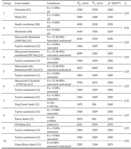
In order to examinethe effective ofthe quantitative prediction method of fracture density, ten

266

groups of test models are established to validate the prediction method of fracture density in Tab. 3.

267

Due to the assumptions that the rock skeleton layer and rock fracture layer of a medium are isotropic,

268

homogeneous, and linear elastic, etc. Ten groups of commercial numerical modelsare performed to

269

validate the application effect of the proposed method in this paper. Each group of test model

270

contains two different core samples. Moreover, the core sample with high velocity and density is

271

defined as a skeleton layer, and the low is defined as a fracture layer, which is conform to the

272

assumptions in Sec. 2.1. As a result, each group of model can be used as a double-layer model. Tab.

273

3 compiles and condenses the virtually published core samples to establish test models [11,50-51], in

274

which contains the core sample testing conditions and some related materials, including the P-wave

275

velocity (

V

_P), the S-wave velocity (

V

_S), the density (



) and the fracture density (



).

276

(11)

Table 3 The core sample parameters of models

278

Group Core sample Conditions

V

P (m/s)

V

S (m/s)



(kg/m3)



1

Dolomite [51] Peff = 0 MPa

air 5200 2700 2450

0.25 Shale [51] Peff = 0 MPa

air 2900 1400 2340

2

Sandy mudstone [50] Peff = 0 MPa

air 4583 2438 2599

0.25 Mudstone [50] Peff = 0 MPa

air 3619 1920 2629

3

Mesaverde Mudshale (1949.3m) [11]

Peff = 27.58 MPa

Saturated undrained 4529 2703 2520

0.25 Taylor sandstone [11] Peff = 0 MPa

saturated 3368 1829 2500

4

Mesaverde immature sandstone(1507.5m) [11]

Peff = 27.58 MPa

saturated undrained 4099 2346 2450

saturated 3368 1829 2500

5

Mesaverde silty limestone(1667.1m) [11]

Peff = 27.58 MPa

saturated 3368 1829 2500

6

Mesaverde Clayshale (1785.7m) [11]

Peff = 27.58 MPa

saturated 3368 1829 2500

7

Taylor sandstone [11] Peff = 0 MPa

saturated 3368 1829 2500

0.25 Dog Creek shale [11] in situ

z=143.3m 1875 826 2000

8

saturated 3368 1829 2500

0.25 Pierre shale [11] in situ

z=450m 2074 869 2250

9

Oil Shale [11] unknown 4231 2539 2370

saturated 3368 1829 2500

10

saturated 3368 1829 2500

0.25 Green River shale [11] Peff=0 MPa

Abbreviations: Peff represents effective stress under triaxial compression; air denotes natural unsaturated state;

279

in situ indicates in-situ measurement.

280

4.2 Validation model forward

281

Tab. 3 provides ten groups of model, which are regard as the double-layer model. Thus, the

282

physical parameters of the models can be calculated according to the above Eqs. in Sec. 2. Tab. 4

283

shows the fast S-wave velocity (

V

_Fast), the slow S-wave velocity (

V

_Slow), the P-wave RMS velocity (

284

P

V

), the S-wave RMS velocity (

V

S), the average density (



all), the coefficient a, and the coefficient b,

285

which are calculated with the Eq. (2), Eq. (3), Eq. (6), Eq. (7), Eq. (12), Eq. (10), and Eq. (11), respectively.

286

Actually speaking, the fast S-wave velocity, slow S-wave velocity, P-wave RMS velocity, S-wave RMS

287

velocity of the prospecting stratum can be obtained from a conventional data processing of

288

(12)

coefficient b can be achieved from the core analysis and logging data of survey area. Finally, the

290

fracture density (



) is predicted by the method of fracture density through solving the Eq. (2), Eq.

291

(3), Eq. (7), Eq. (12), and Eq. (13).

292

Table 4 The physical parameters of models

293

Group

V

Fast (m/s)

V

Slow (m/s)

V

P (m/s)

V

S (m/s)



all (kg/m3) a b

1 2450 2068 4480 2281 2423 1.622 1.793

2 2318 2272 4319 2296 2607 1.776 1.906

3 2514 2373 4204 2449 2515 1.727 1.845

4 2226 2179 3902 2204 2463 1.722 1.845

5 2681 2456 4507 2580 2598 1.761 1.845

6 2017 2002 3683 2010 2545 1.834 1.845

7 1669 1242 2900 1488 2375 1.845 1.709

8 1658 1316 2978 1509 2438 1.845 1.875

9 2375 2296 3996 2338 2402 1.653 1.845

10 1816 1805 3349 1814 2394 1.845 1.541

4.3 Results

294

According to the quantitative prediction method of fracture density in Sec. 2.5 and the

295

aforementioned physical parameters of models in Tab. 4, we can predict the fracture density (



).

296

Moreover, we used the quasi-Newton method to solve the Eq. (2), Eq. (3), Eq. (7), Eq. (12), and Eq.

297

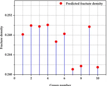
(13) for predicting the fracture density in this study. Fig. 5 shows the predicted values of the fracture

298

density (



'). It can be seen that the predicted fracture density is 0.24-0.25 for the ten models, which

299

indicates the effective of the predicted values for the fracture density. The minimum value located in

300

the seventh model, with a value of about 0.241,and the maximum value, 0.249 is located in the fourth

301

model.

302

303

Figure 5. The predicted fracture density.

304

In addition to the predicted values for the fracture density, the root-mean-square error (RMSE)

305

and absolute relative deviation (ARD) were used as indexes to evaluate the prediction effects. The

306

smaller the root-mean-square (RMSE) and ARD were, the more favorable the prediction effect was.

307

The root-mean-square error (RMSE) was used to weight the deviation between the prediction result

308

and the actual value, and its calculation Eq. was Eq. (23).The ARD was usually used to evaluate the

309

accuracy of method through comparing the prediction value and the actual value. Its calculation Eq.

310

is Eq. (24), as follows:

311

0 2 4 6 8 10

0.240 0.244 0.248 0.252

Group number

Fra

cture

de

nsity

(13)



_'



2 1

n

i i i

RMSE

n

 









(23)

312

'

100

i i

i

ARD

 









i



1, 2,...,

n

(24)

313

In Eq. (23) and Eq. (24),



i' represents the prediction fracture density;



i denotes the actual fracture

314

density; and n indicates the number of the validation models.

315

316

Figure 6. The RMSE and ARD of the predicted fracture density.

317

Fig. 6 shows the results of RMSE and ARD. It was shown thatARD were less than 5% and RMSE

318

was 4.88×10-3_{. It indicated that the fracture density predicted by the method developed in this study}

319

were in agreement with the actual data. The results demonstrated that the quantitative prediction

320

method proposed in this study was capable for predicting fracture density data.

321

In this study, for establishing a practical method to predict the fracture density quantitatively,

322

we assume that a thin interbedded medium is composed of two components: rock skeleton layer

323

(matrix) and rock fracture layer (including filling, water, oil, and gas), and the rock skeleton layer

324

and rock fracture layer of the thin interbedded medium are isotropic, homogeneous, and linear elastic,

325

etc., which is an idealized hypothesis. As a result, the thin interbedded medium can equivalent to the

326

double-layer medium under these assumptions. Actually speaking, these assumptions will involve

327

in deviation to this method, and the effect of these assumptions on the prediction method of fracture

328

density will be the focus in the future research. However, it is significant that the new method can

329

provide a scale in predicting the fracture density. Besides, the new method can be applied to the

330

Hudson model, and then the scope of the prediction method of fracture density is extended, which

331

is verified in Sec. 3.

332

Based on the above assumptions, the relationships between fracture density and the seismic

333

response is established. In Sec. 2.2-2.3, we use the fast S-wave velocity, the slow S-wave velocity, the

334

P-wave RMS velocity, and the S-wave RMS velocity as constraints to predict the fracture density,

335

which can be obtained from a conventional data processing of multicomponent seismic exploration.

336

Therefore, the processing quality of the multicomponent data will affect the application of the

337

prediction method for fracture density. Besides, only concerns the wave velocity as a function of

338

density in Sec. 2.4 is imprecise, which is to simplify the prediction method. In fact, the velocity is

339

related to several factors among which for instance the Young’s modulus. Moreover, there will be an

340

error in predicting the average density of a target layer by the core analysis and logging data. The

341

influence of these factors on the prediction results will be reported in the later article.

342

5. Conclusions

343

The accurate prediction of fracture density plays an important role in the exploration and

344

development of unconventional reservoirs which have received widespread interest in recent years.

345

0 2 4 6 8 10

-2 -1 0 1 2 3 4 5

Group number

A

R

D

(%

)

ARD

(14)

In this study, we consideredthat a thin interbedded medium is composed of the rock skeleton layer

346

and rock fracture layer, besides the rock skeleton layer and rock fracture layer are isotropic,

347

homogeneous, and linear elastic, etc. Under the above assumptions, the thin interbedded medium

348

can be equivalent to a double-layer medium, and then the relationships between the fracture density

349

and the physical parameters of a target layer, such as the fast S-wave velocity, the slow S-wave

350

velocity, the root mean square (RMS) velocity, and the density, were established, which makes up

351

the gap between the fracture density and the seismic response. While, a quantitative prediction

352

method for fracture density was proposed. Afterwards, the Hudson model was used to test the

353

applicability of this method. The result shown that the new method can be applied to the Hudson

354

model. Moreover, the quantitative prediction method of fracture density was used tothe ten groups

355

of validation model, in which RMSE and ARD were as the index of evaluation. The RMSE=4.88×10

-356

3_{demonstrated that the fracture density predicted by the} _{method developed in this study are in}

357

satisfactory agreement with the actual data. Meanwhile, the ARD of the fracture density were less

358

than 5%, which indicated that this method can accurately predict fracture density. All in all, a

359

powerful method for predicting fracture density is proposed in this study, and the method can be

360

used topredict the fracture density of unconventionalreservoirs, which provided a new idea for the

361

study of reservoirs fracture.

362

Acknowledgments: This research is financially supported by the National Science and Technology Supporting

363

Program (2012BAB13B01), National Key Scientific Instrument and Equipment Development Program

364

(2012YQ030126), National Natural Science Foundation of China (41504041).

365

Author Contributions: Suping Peng was the director of the project. Dengke He proposed the idea of the method.

366

Liang Sun was responsible to build the method, models and write this draft. Shu Wang made some constructive

367

suggestions for the test data.

368

Conflicts of Interest: The authors declare no conflict of interest.

369

Nomenclature

370

a Coefficient between the P-wave velocity and the density for the skeleton layer (dimensionless)

b Coefficient between the P-wave velocity and the density for the fracture layer (dimensionless)

C Stiffness tensor (N/m2₎

CH _{Stiffness tensor of Hudson model (N/m}2₎

d1 Volume of the skeleton (m3)

𝑑1𝐻 Volume of the skeleton in Hudson model (m3)

d2 Volume of the fracture (m3)

𝑑2𝐻 Volume of the fracture in Hudson model (m3)

f1 Volumetric proportion between the skeleton layer and the total layer (dimensionless)

f2 Volumetric proportion between the fracture layer and the total layer (dimensionless)

Peff Effective stress (MPa)

t1 Vertical propagation time of P-wave in the skeleton layer (s)

t2 Vertical propagation time of P-wave in the fracture layer (s)

VFast Fast S-wave velocity (m/s)

VG P-wave velocity in Gardner empirical formula (m/s)

VP P-wave velocity (m/s)

𝑉𝑃

̅̅̅ _{Root mean square velocity of P-wave (m/s)}

(15)

𝑉𝑃1𝐻 P-wave velocity of the skeleton in Hudson model (m/s)

VP2 P-wave velocity of the fracture (m/s)

𝑉𝑃2𝐻 P-wave velocity of the fracture in Hudson model (m/s)

VS S-wave velocity (m/s)

𝑉̅𝑆 Root mean square velocity of S-wave (m/s)

VS1 S-wave velocity of the skeleton (m/s)

𝑉𝑆1𝐻 S-wave velocity of the skeleton in Hudson (m/s)

VS2 S-wave velocity of the fracture (m/s)

𝑉𝑆2𝐻 S-wave velocity of the fracture in Hudson (m/s)

VSlow Slow S-wave velocity (m/s)

Greek letters

371

𝛼 Fracture width ratio (dimensionless)

𝜀 Fracture density (dimensionless)

𝜀𝐻 _{Fracture density of Hudson model (dimensionless)}

𝜀′ _{Prediction value of fracture density (dimensionless)}

ρ Density (Kg/m3₎

ρ1 Density of the skeleton (Kg/m3)

𝜌1𝐻 Density of the skeleton in Hudson model (Kg/m3)

ρ2 Density of the fracture (Kg/m3)

𝜌2𝐻 Density of the fracture in Hudson model (Kg/m3)

ρall Average density (Kg/m3)

ρG Density in Gardner empirical formula (Kg/m3)

References

372

1. Montgomery, S.L.; Jarvie D.M.; Bowker, K.A.; Pallastro, R.M. Mississippian Barnett shale, Fort Worthbasin,

373

north-central Texas: Gas-shale play with multitrillion cubic foot potential. AAPG Bulletin 2005, 90, 963-966,

374

doi: 10.1306/09170404042.

375

2. Dang, W.; Zhang, J.C.; Tang, X.; et al.Investigation of gas content of organic-rich shale: A case study from

376

Lower Permian shale in southern North China Basin, central China. Geoscience Frontiers 2018, 9, 559-575,

377

doi: 10.1016/j.gsf.2017.05.009.

378

3. Wang, Y.; Zhu, Y.M.; Liu, Y.; Chen, S.B. Reservoir characteristics of coal-shale sedimentary sequence in

379

coal-bearing strata and their implications for the accumulation of unconventional gas. Geoscience Frontiers

380

2018, 9, 559-575, doi.org/10.1016/j.gsf.2017.05.009. Journal of Geophysics and Engineering 2018, 15, 411-420,

381

doi: 10.1088/1742-2140/aa9a10.

382

4. Wang, X.Z.; Zhang, L.X.; Jiang, C.F.; Fan, B.J. Hydrocarbon storage space within lacustrine gas shale of the

383

Triassic Yanchang Formation, Ordos Basin, China. Interpretation 2015, 3, SJ15-SJ23, doi:

10.1190/INT-2014-384

0125.1.

385

5. Saidian, M.; Ghazanfari, M.H.; Masihi, M.; Kharrat, R. Five-spot injection/production well location design

386

based on fracture Geometrical Characteristics in Heavy Oil Fractured Reservoirs during Miscible

387

Displacement: An Experimental Approach. Chemical Engineering Communications 2012, 199, 306-320, doi:

388

10.1080/00986445.2011.577849.

389

6. Johansen, T.A.; Jensen, E.H.; Mavko, G.; Dvorkin, J. Inverse rock physics modeling for reservoir quality

390

prediction. Geophysics 2013, 78, M1-M18, doi: 10.1190/GEO2012-0215.1.

391

7. Far, M.E.; Hardage, B.; Wagner, D. Fracture parameter inversion for Marcellus Shale. Geophysics 2014, 79,

392

C55-C63, doi: 10.1190/GEO2013-0236.1.