Electronic Thesis and Dissertation Repository
11-8-2013 12:00 AM
Application of Computer Algebra in List Decoding
Application of Computer Algebra in List Decoding
Muhammad Foizul Islam Chowdhury The University of Western Ontario
Supervisor Eric Schost
The University of Western Ontario Graduate Program in Computer Science
A thesis submitted in partial fulfillment of the requirements for the degree in Doctor of Philosophy
© Muhammad Foizul Islam Chowdhury 2013
Follow this and additional works at: https://ir.lib.uwo.ca/etd
Part of the Digital Communications and Networking Commons, and the Theory and Algorithms Commons
Recommended Citation Recommended Citation
Chowdhury, Muhammad Foizul Islam, "Application of Computer Algebra in List Decoding" (2013). Electronic Thesis and Dissertation Repository. 1851.
https://ir.lib.uwo.ca/etd/1851
This Dissertation/Thesis is brought to you for free and open access by Scholarship@Western. It has been accepted for inclusion in Electronic Thesis and Dissertation Repository by an authorized administrator of
(Thesis format: Paper)
by
Muhammad Foizul Islam Chowdhury
Graduate Program in
Computer Science
A thesis submitted in partial fulfillment of the requirements for the degree of
Doctor of Philosophy
The School of Graduate and Postdoctoral Studies Western University
The amount of data that we use in everyday life (social media, stock analysis, satellite communication, etc.) is increasing day by day. As a result, the amount of data that needs to traverse through electronic media as well as to store are rapidly growing and there exist several environmental effects that can damage these important data during travelling or while in storage devices. To recover correct information from noisy data, we use error correcting codes. The most challenging work in this area is to have a decoding algorithm that can decode the code quite fast and that can tolerate highest amount of noise, so that we can use it in practice.
List decoding has been an active research area for last two decades. This re-search popularise in coding theory after the breakthrough work by Madhu Sudan where he used list decoding technique to correct errors that exceed half the minimum distance of Reed Solomon codes. Towards the direction of code development that can reach theoretical limits of error correction, Guruswami-Rudra introduced folded Reed Solomon codes that reached at 1−R−ǫ for ǫ >0. To decode these codes, one has to first interpolate a multivariate polynomial and then to factor out all possible roots. The difficulties that lie here are efficient interpolation, dealing with multiplic-ities smartly, and efficient factoring. This thesis deals with all these cases in order to have practical folded Reed Solomon codes.
Keywords. List Decoding, Structured matrix multiplication, Newton-Pueisux ex-pansion, Newton-iteration.
I would first like to thank my thesis supervisor Associate Professor ´Eric Schost in the Department of Computer Science at Western University, Canada. The door to Prof. ´Eric Schost office was always open whenever I ran into a trouble spot or had a question about my research or writing. He consistently helped me on the way of this thesis and steered me in the right direction whenever he thought I needed it. I am grateful to him for his excellent support to me in all arenas.
Sincere thanks and appreciation are extended to all the members from our Ontario Research Centre for Computer Algebra (ORCCA) lab and the Computer Science Department for their invaluable teaching and assistance.
My deep gratitude goes to my parents along with all my brothers, sisters, sister-in-laws, brother-sister-in-laws, nieces and nephews. Special thanks goes to my brother Dr. Badrul Islam Choudhury and Sister-in-law Sabiha Choudhury Moona. My heartfull thanks goes to my two cutest nieces Manha and Rahmah who provided me lots of recreation during heavy workload.
Abstract ii
Acknowledgments iii
1 Introduction 1
1.1 Error correcting codes . . . 2
1.2 Reed-Solomon codes . . . 3
1.3 Problem statement and overview of our results . . . 6
Bibliography . . . 8
2 Mathematical preliminaries 10 2.1 Introduction . . . 10
2.1.1 Group . . . 10
2.1.2 Ring . . . 11
2.1.3 Field . . . 11
2.1.4 Notion of Finite field . . . 12
2.1.5 Polynomial multiplication . . . 14
2.1.6 Matrix structure . . . 14
Bibliography . . . 16
3 Complexity of MultivariateInterpolation with Multiplicities 17 3.1 Introduction . . . 18
3.2 Preliminaries: assumption H1 . . . 25
3.3 Solving structured linear systems . . . 26
3.4 Reducing Problem 1 to Problem 2 . . . 29
3.5 Solving Problem 2 through a mosaic-Hankel linear system . . . 32
3.6 A direct solution to Problem 2 . . . 37
Bibliography . . . 41
4.2 Basics on structured linear systems . . . 46
4.3 Structured matrix inversion . . . 49
4.3.1 Matrix inversion using block Gaussian elimination . . . 50
4.3.2 Structured matrix inversion . . . 51
4.4 Structured matrix multiplication. . . 54
Bibliography . . . 58
5 Power Series Solutions of Singular (q)-Differential Equations 61 5.1 Introduction . . . 61
5.2 Divide-and-Conquer . . . 67
5.3 Newton Iteration . . . 72
5.3.1 Gauge Transformation . . . 72
5.3.2 Polynomial Coefficients . . . 73
5.3.3 Computing the Associated Equation . . . 74
5.3.4 Solving the Associated Equation. . . 75
5.4 Implementation . . . 79
Bibliography . . . 81
6 Polynomial Root-Finding for Nonlinear Equations 84 6.1 Introduction . . . 84
6.2 The classical case (s = 1). . . 85
6.2.1 Root-finding when m= 1 . . . 86
6.2.2 Root-finding when m >1 . . . 87
6.3 The folded case (s >1) . . . 93
6.3.1 The linear case . . . 94
6.3.2 The regular case . . . 96
6.3.3 The general case . . . 98
6.4 A heuristic . . . 102
Bibliography . . . 104
7 Conclusions and future work 108 7.1 Future work . . . 110
1 MBA algorithm invert Toeplitz-like matrices. . . 53
2 Mul Rec(U,V,W, n, ν,α, µ¯ ) . . . 56
3 Mul(U,V,W, n, α) . . . 56
4 Recursive Divide-and-Conquer . . . 68
5 Divide-and-Conquer . . . 70
6 PolCoeffsDE . . . 74
7 Solving Eq. (5.10) when k = 1 or q6= 1 . . . 76
8 Solving Eq. (5.10) when k > 1 andq = 1 . . . 77
9 Newton iteration for Eq. (5.8) . . . 78
10 Roth & Ruckenstein(M, k, ψ, i) . . . 88
11 Newton-Puiseux expansion(Q, k, ψ, i) . . . 90
12 RDAC(A0, . . . , As, γ, i, ℓ) . . . 95
13 Root Computation(Q, s, k, γ) . . . 97
14 Filter(Q, f, k, γ) . . . 98
15 Newton-Puiseux expansion(Q, i, k, ψ) . . . 101
16 Lift root from fRS Q(Q, s, k, γ) . . . 102
1.1 A simple communication system. . . 1
1.2 Folded Reed-Solomon code fors = 4. . . 4
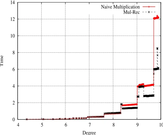
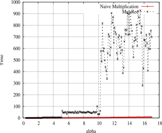
4.1 AlgorithmMul Rec vs naive reduction . . . 59
4.2 α fixed . . . 59
4.3 Degree fixed . . . 60
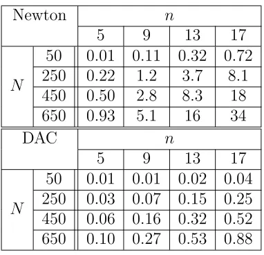
5.1 Timings with n = 1, k= 1, q6= 1 . . . 80
5.2 Timings with k = 1, q6= 1 . . . 80
6.1 Execution of Roth and Ruckenstein’s algorithm . . . 89
6.2 The Newton polygon of polynomial Q . . . 89
6.3 Execution of the Newton-Puiseux algorithm . . . 91
6.4 Newton polygon . . . 99 6.5 Timing between our algorithm and Beelen and Brander’s algorithm . 104
2.1 Addition modulo 1 +x+x3 . . . . 13
2.2 Multiplication modulo 1 +x+x3 . . . . 14
3.1 Overview of previous results, s= 1. . . 22
5.1 Timings with k = 3, q6= 1 . . . 81
6.1 Number of times a new polynomial Q was needed . . . 103
6.2 Timing of Interpolation and Root-Computation . . . 104
Chapter 1
Introduction
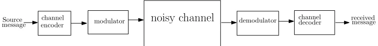
In everyday life, large amounts of data travel through various electronic comminica-tion channels. The amount of data is increasing and no communicacomminica-tion channel or storage device is error prone: errors can be introduced to these data while they are traversing wired or wireless media and corrupt them; these data can also be damaged while we store them in electronic media like hard disks or CDs / DVDs due to the presence of bad sectors or scratches. The solution to this problem is to apply a coding scheme, so that we can recover correct information even in the presence of errors in the data. Coding theory deals with this question.
A simple communication system is depicted in Figure1.1; the main source of error is the noisy channel. To recover the correct information that passed through the noisy channel, coding schemes add some redundancy to the original data: if we want to transfer k symbols through the noisy channel, our codding scheme will encode these symbols into n (for n > k) symbols, by adding n−k redundant symbols. These n
symbols will then traverse the noisy channel, and we expect that the receiver will be able to recover the original symbols correctly, as long as the number of errors falls within some error limits. Both the decoder and encoder use error correcting codes to perform these operations.
Source
message encoder
channel modulator noisy channel demodulator channel
decoder receivedmessage
1.1
Error correcting codes
Error correcting codes tell us about how to add redundant symbols to the original data so that the receiver can recover the original message even if they received corrupted symbols. The following definitions taken from [4] are essentials for error correcting codes.
• Encoding: An injective functionE :δk→δnhaving parametersk,n ∈Nthat
maps a message m consisting of k symbols over some alphabet δ (for example the binary alphabet δ = {0,1}) into a string E(m) of length n over δ, where
n > k,is known as an encoding. The word that is encoded by this function, i.e.
E(m), is referred as a codeword. If |δ| is finite then the alphabet size is often written q =|δ|.
• Decoding: The sender sends the encoded codeword E(m) through the noisy channel. The receiver may receive a distorted copy of the transmitted codeword, so she needs to figure out the original message. This role is done by a decoding function, D : δn → δkS{1}, which maps the codeword of length n, which is
possibly corrupted, to a string of length k.
• Error-Correcting code: It is the set of all codewordsC ⊂ δnthat are obtained
by encoding messages, i.e. the image of the encoding functionE. Each codeword in C has the same length n, so we say that C is a block code of length n. If C ⊆ δn is a block code of length n with q = |δ| finite, we say that C is a q-ary
(error-correcting) code and the dimension of this code C is k = logq|C|.
• Rate: The ratioR = kn of the number of symbols in a message to the length of the encoding map in the above definitions is called the rate of the code. This measures the amount of redundancy that is added by the encoding.
• Distance: Given two vectorsxandyof lengthn, with entries inδ, thedistance
between these two vectors is the number of coordinates that differ from each other, i.e. {i|xi 6=yi}. Theminimum distance (or simply, distance) of a code is
defined to be the smallest distance between two distinct codewords; according to the Singleton bound,the minimum distance d of a code C cannot be greater thann−k+ 1 andmaximum distance separable(or MDS) codes are codes that remain within this bound.
subspace of an n-dimensional vector space over F; such codes are known as a linear
q-array codes. Here the dimension of the code k = logq|C| matches the vector space dimension as an F-subspace of Fn. A linear code having length n dimension k and minimum distance d is also known as an [n, k, d]q code.
Depending on the number of errors, decoding strategies are available: typically, one can consider unique decodingorlist decoding. In the former, the decoder outputs a single candidate for the message; this may be feasible only when few errors occured. List decoding is an alternative approach, due to Elias [3], which returns a list of candidates, one of which is the correct message. In this thesis, we will focus on list decoding algorithms for a particular family of codes, Reed-Solomon codes, which we introduce now.
1.2
Reed-Solomon codes
There exist many linear codes; Reed-Solomon codes are one of the most famous ones in coding theory, and will be the main focus of this thesis.
Definition 1. (Reed-Solomon Codes) Let F be a field with at least n elements,
and consider n pairwise distinct values α = (α1, . . . , αn) ∈ Fn. Given a polynomial
f(x) =Pii==0k−1δixi in F[x], where δi ∈F are the message symbols, the Reed-Solomon codeword (y1, . . . , yn) associated to f is obtained by evaluating f(x) at α, so that
yi =f(αi). This code is denoted
RSq(n, k, α) ={(f(α1), . . . , f(αn)) | f ∈F[x]k},
where F[x]k is the set of polynomials having coefficients in the base field Fand degree
less than k.
Although not strictly necessary, it will be convenient to take α of the form 1, γ, . . . , γn−1, for some γ in F\ {0} of multiplicative order at least n (often, by a slight abuse of expression, we may refer toγ as a primitive element, although strictly speaking this would be the case only if |F|=n+ 1).
Since a nonzero polynomial of degree less thankcan have at mostk−1 zeros, every nonzero codeword will have at least n−k+ 1 nonzero components. The minimum distance of RSq(n, k, α) is equal to n−k+ 1,which is the singleton bound, so
Reed-Solomon codes are maximum distance separable.
the number of errors that can be corrected by a decoder should be as close ton−k as possible; that is, error correction should be possible as long as k symbols are correct. The fraction of errorsρis defined as the ratio of the number of errors to the length; the information theoretic limit states that this number is at most (n−k)/n = 1−R [5]. Standard unique decoding techniques, using for instance the Berlekamp-Massey algorithm, recover the correct message from the codeword and can decode the correct message as long as the number of erros is less than (n−k)/2. Folded Reed-Solomon
codes, invented by Guruswami and Rudra [5] following previous work by Parvaresh
and Vardy [9], are derived from Reed-Solomon codes and can tolerate an error ratio of 1−R−ε for any ε >0 (using list decoding techniques).
These codes rely on a folding process, characterized by a folding parameters>1.
For the folded case, we will make from the outset the assumption that the evaluation points (α1, . . . , αn) are of the form (1, γ, . . . , γn−1).
Definition 2. (Folded Reed-Solomon codes) Let s, n be integers such that s
divides n; let F be a field with at least n elements, and consider n pairwise distinct
values α = (1, γ, . . . , γn−1) ∈ Fn. Given a polynomial f(x) = Pi=k−1
i=0 δixi in F[x],
where δi ∈ F are the message symbols, the folded Reed-Solomon codeword associated
to f consists in the n/selements Y1, . . . , Yn/s, with yi∈Fs given by
Yi = (y(i−1)s+1, . . . , y(i−1)s+s), yi =f(αi).
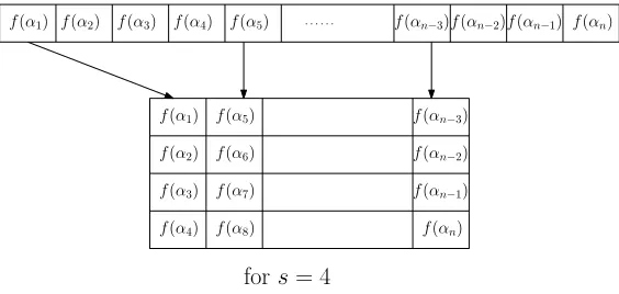
In other words, the symbols in the codeword are now s-uples of values in F, obtained by juxtaposing s consecutive “elementary symbols” f(γi). When s= 1, we
recover Reed-Solomon codes; Figure 1.2 gives an example of folded Reed-Solomon code taken from [5], where the folded parameter s is equal to 4.
f(α1) f(α2) f(α3) f(α4) f(α5) . . . f(αn−3)f(αn−2)f(αn−1) f(αn)
f(α1)
f(α2)
f(α3)
f(α4)
f(α5)
f(α6)
f(α7)
f(α8)
f(αn−3)
f(αn−2)
f(αn−1)
f(αn)
fors= 4
Figure 1.2: Folded Reed-Solomon code for s = 4.
Rudra) that for any ε > 0 and rate R < 1, there exists a family of folded Reed-Solomon codes that have rate at leastRand which can belist decodedup to a fraction 1−R−ε of errors in an efficient manner. We recall below some of the landmark results in this direction.
Recall first that unique decoding for Reed-Solomon codes can accommodate up to (n−k)/2 errors, or equivalently a ratio of (1−R)/2 = 1−(R+ 1)/2.
The first crucial step toward incorporating a larger error ratio was solved by Madhu Sudan [10], using list decoding techniques. In a nutshell, Sudan’s algorithm recovers a (small) list of polynomials that contains the message, provided the error ratio is at most 1−√2R. The following shows the main step in Sudan’s list decoding algorithm; they form the blueprint of all algorithms that follow.
• Interpolate a bivariate polynomial Q(x, y) such that Q(αi, yi) = 0 (under
suit-able degree bounds [10]).
• Find all polynomials f(x) such that y−f(x) is a factor of Q.
• Keep those where f(αi) =yi for at least n−e values of i, where e is a bound
on the number of errors and the degree off is less than k.
Correctness of this algorithm follows from imposing suitable degree bounds on Q; we will not need to state these bounds below.
This work was further developed by Guruswami and Sudan in [6] by introducing
multiplicities: Qmust vanish at high enough order at the points (αi, yi). For suitable
choices of the degree bounds on Q and the multiplicity parameter, Guruswami and Sudan’s algorithm allows error ratios up to 1−√R [6].
Following the work of Guruswami and Sudan, Parvaresh and Vardy developed codes that can tolerate errors, and can be seen as precursors of the folded codes we defined above. Again, the algorithm proceeds through two main steps, evaluation and root-finding.
Finally, in 2008, Guruswami and Rudra introduced in [5] the folded Reed-Solmon codes defined above, by formulating a relation between Reed Solomon codes and Parvaresh and Vadry codes; their list-decoding algorithm works as follows:
• Compute a multivariate polynomialQ(x, z1, . . . , zs) such that, fori= 0, . . . , n−
1,
at orderm (that is, all derivatives ofQ of order up to m vanish as well at this point). Here, α1, . . . , αn are the evaluation points and y1, . . . , yn are the values
as in Definition 2.
• Find all polynomials f(x) such that Q(x, f(x), f(γx), . . . , f(γs−1x)) = 0. • Keep all polynomials f such that f(αi) = yi for at least (n −e) consecutive
values of i∈n.
As for Sudan’s algorithm, Qis subject to some degree constraints: upper bounds are given for its total degree, as well as for is weighted degree, for a weight where every variable zi has degree k−1. It will not be necessary for us to make these constraints
explicit; Guruswami and Rudra’s article gives all details. To conclude, remark that when s= 1, no folding occurs and we recover Sudan’s algorithm.
1.3
Problem statement and overview of our results
In this work, we consider the two main steps highlighted in the above description of the Sudan / Guruswami-Sudan / Guruswami-Rudra list decoding algorithms: inter-polation and root-finding. Although we saw that they are rooted in coding theory, these problems can be stated independently of the framework of error correction; this is the point of view we adopt, considering these questions as interesting by themselves.
Interpolation. The first question is to recover a polynomial Q that satisfies con-straints (1.1), under additional requirements on its total degree and its weighted degree, for a well-chosen weight.
This is a linear algebra problem; as such, most early references on the subject (such as Sudan’s and Guruswami-Sudan’s papers) point out that this problem can be solved using essentially Gaussian elimination. Much work has been devoted to improve on naive linear algebra techniques: standard techniques now employ either fast linear algorithms, or polynomial lattice reduction techniques.
Chapter 3 gives a review of the existing literature and presents a new algorithm, inspired by previous work by Zeh, Gentner and Augot [11], which is the fastest to date (to the best of our knowledge).
Root-finding. The second main question is to find all polynomials f that satisfy an equation of the type
Q(x, f(x), f(γx), . . . , f(γs−1x)) = 0, (1.2) for someQinF[x, z1, . . . , zs]. When s= 1, this means thatf satisfiesQ(x, f(x)) = 0, so we are left with a bivariate factorization problem, for which standard solutions ex-ist. For higher values ofs, the solution proposed by Guruswami and Rudra (following previous work by Parvaresh-Vardy) is the following.
Assume that γ has multiplicative order preciselyq−1, with q=|F|, letP be the irreducible polynomialP(x) =xq−1−1, and letF′ =F[x]/P. Then, Guruswami and Rudra prove that f can be recovered as a root of
T =Q(x, z, zq, . . . , zq(s−1)),
seen as a univariate polynomial in F′[z]. However, the large degree of this polynomial in z makes this approach very expensive in practice.
Following previous work by Pecquet and Augot for the Guruswami-Sudan case [1], we investigate how lifting techniques can be used to compute power series(and thus polynomial) solutions of (1.2).
Equations such as (1.2) are often called q-difference equations, although in our context we should call them γ-difference equations (traditionally, the scaling factor is written as q rather than as γ; this goes back to at least [8]). It turns out that such equations are very similar to differential equations; the analogy can be seen by noting that, if we were in a context were we could let γ approach 1,
lim
γ→1
f(γx)−f(x) (γ−1)x =f
′(x) for any polynomial f. As
f(γx)−f(x) (γ−1)x =
P
ifi(γi−1)xi
(γ−1)x
that becomes f′(x) when γ →1.
In Chapter 5, we give algorithms that handle simultaneously differential and q -difference cases, using either Newton iteration or divide-and-conquer techniques, in the simplest case whereQis linear inz1, . . . , zs. Previous algorithms existed to handle
results to (some) singular cases and to the q-difference case (which is needed in our applications to list-decoding).
In Chapter 6, we describe the case of arbitrary Q. When s = 1, well-known techniques involve a combination of Newton iteration (when the solutions have no multiplicity) and of a desingularization process called the Newton-Puiseux algorithm in general. We show how these techniques extend to the folded case, and using recent work by Cano and Fortuny Ayuso [7] we propose a heuristic that drastically simplifies the resolution process.
Bibliography
[1] D. Augot and L. Pecquet. A Hensel lifting to replace factorization in list-decoding of algebraic-geometric and Reed-Solomon codes. IEEE Transactions on
Infor-mation Theory, 46(7):2605–2614, 2000.
[2] A. Bostan, C.-P. Jeannerod, C. Mouilleron, and ´E. Schost. Fast simultaneous multiplication of a structured matrix by vectors. PrePrint, 2012.
[3] P. Elias. List decoding for noisy channels. Technical Report 335, pages 94–104, September-1957.
[4] V. Guruswami. List decoding of error-correcting codes, volume 3282 of Lecture
Notes in Computer Science. Springer-Verlag, 2005.
[5] V. Guruswami and A. Rudra. Error correction up to the information-theoritic limit. Communications of the ACM, 52(3):87–95, 2009.
[6] V. Guruswami and M. Sudan. Improved decoding of Reed-Solomon and algebraic-geometric codes. IEEE Transactions on Information Theory, 45(6):1757 – 1767, Sep–1999.
[7] P. Fortuny Ayuso J. Cano. Power series solutions of non-linearq-difference equa-tions and the Newton-Puiseux algorithm, 2012. arXiv:1209.0295.
[8] F. H. Jackson. q-difference equations. American Journal of Mathematics, 32(4):pp. 305–314, 1910.
[10] M. Sudan. Decoding of Reed-Solomon codes beyond the error-correction bound.
Journal Of Complexity, 13:180–193, 1997.
[11] A. Zeh, C. Gentner, and D. Augot. An interpolation procedure for list decoding ReedSolomon codes based on generalized key equations. IEEE Transaction on
Chapter 2
Mathematical preliminaries
This chapter discusses about various mathematical basics that was used through out the thesis.
2.1
Introduction
This chapter begins with the description of field, ring, group. Then we describe about several structured matrix that act as basic for solving our linear system. The presentation of this part follows [1].
2.1.1
Group
A group is a set of elements with a binary operation ⋄that have following properties. Usually the group is denoted by {G,⋄}.
1. Closer: a⋄b∈ G ⇐⇒a,b∈ G.
2. Associativity: a⋄(b⋄c) = (a⋄b)⋄c ∀a,b,c∈ G.
3. Commutativity: a⋄b=b⋄a∀a,b∈ G.
4. Identity element: The group G has an element e for which we have a⋄e = e⋄a=a∀a∈ G. The element eis known as identity element of that group.
5. Inverse element: there exist an element a′ ∈ G for each a ∈ G such that a⋄a′ =a′ ⋄a=ei.e. identity element.
A groupG is said to be cyclic when each element of that group can be represented as a power of an element of that group. Let a be an element of a group G, then
by means of powering of an element of that group, we refer that number of group operations, e.g. a3 = a⋄ a⋄ a. The element of a group G which can be used to
represent all element ofG by this powering operation is known as a primitive element of that group G.It is also called generator of the group G.
2.1.2
Ring
A ring is a set of elements with two binary operations addition and multiplication that have following properties. We represent a ring by {R,+,×},
1. A ring R have all the properties of a group. IfR is an additive group then 0 is it’s identity element and −ais the inverse of an element a∈ R.
2. Closure under multiplication: a,b∈ R ⇒a×b∈ R.
3. Commutativity under multiplication: a×b=b×a ∀a,b∈ R.
4. Associativity under multiplication: ∀a,b,c ∈ R; we have a×(b×c) = (a× b)×c.
5. Distributivity: ∀a,b,c∈ R; we have
(a) a×(b+c) = (a×b) + (a×c)
(b) (a+b)×c= (a×c) + (b×c)
An integral domain is a commutative ring that have following properties in addi-tion to the properties of a ring R.
• Multiplicative identity: ∀a∈ R, we have 1∈ R such thata×1 = 1×a=a.
• No zero divisor: a×b= 0 ∀a,b∈ R ⇒ eithera= 0 or b= 0.
2.1.3
Field
A field F is a set of elements with two operations addition and multiplication that have following properties.
• Multiplicative inverse: For each element a∈ F \0,we have a−1 ∈ F such that aa−1 =a−1a= 1.
We can do all arithmetic operation, i.e. addition, subtraction, multiplication and division, on a a field F and the result of the operation will be in that field F. Here the division operations is performed as follows
a
b =ab
−1
∀a,b∈ F.
Polynomial Ring
A polynomial ring over a field F, represented by F[x], is a set of polynomials P of the form
P =p0+p1X+p2X2+· · ·+Pm−1Xm−1+PmXm.
where the coefficients of P, p0, . . . , pm, are elements of underlying field F and X is
indeterminate. The degree ofP is the highest power inX that has nonzero coefficient.
2.1.4
Notion of Finite field
Let p be a prime and n is a positive integer, then the number of elements of (also known as order of finite field) a finite field ispn.Herepis said to be the characteristic
of the field. Generally we use GF(pn) or F
pn to denote a finite field having order pn.
GF stands for Galois Field. The structure of the finite field when n > 1 is different than the structure of the finite field when n = 1.
For a prime pand n= 1,the finite field Fp (GF(P)) is the set Zp of integers with arithmetic operation modulo prime p. Here
Zp ={0,1, . . . , p−1}.
Let F be a field, then a polynomial f ∈F[x], that have coefficients over the field F, is said to be irreducible over the field F if and only if f(x) is irreducible as an element over the polynomial ring F[x].
For a prime p and n > 1, the finite field Fpn (GF(Pn)) is defined by using an
Example of finite field of the form Fpn
Let ξ be the set of all polynomials having degree less than n over a field Fp. Each polynomial in this set can be represented by
f(x) =p0+p1X+· · ·+pn−1xn−1
wherepi ∈Fp,for 06i6n−1.It is easily verifiable that the setξ has pn number of
polynomials. The set having this property is a finite field with following arithmetic operations.
• All basic arithmetic operations is executed modulo p for coefficients.
• When the degree of product of two elements from ξ is greater than n, it gets reduced modulo an irreducible polynomial f(x) having degree n;
We gave a simple example of a finite fieldFpn which is taken from [1]. Here we choose
p= 2 and n = 3.
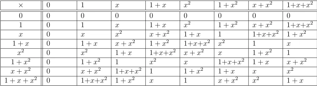
Example of operations on a finite field F23
An irreducible polynomial having degree 3 over F2 isx3+x+ 1 and let the setξ has polynomials of degree less than 3 over F2. Here
ξ={0,1, x,1 +x, x2,1 +x2, x+x2,1 +x+x2}.
The arithmetic operation on this elements modulox3+x+ 1 are shown in following tables 2.1 and table 2.2.
+ 0 1 x 1 +x x2 1 +x2 x+x2 1+x+x2 0 0 1 x 1 +x x2 1 +x2 x+x2 1+x+x2 1 1 0 1 +x x 1 +x2 x2 1+x+x2 x+x2
x x 1 +x 0 1 x+x2 1+x+x2 x2 1 +x2 1 +x 1 +x x 1 0 1+x+x2 x+x2 1 +x2 x2
x2 x2 1 +x2 x+x2 1+x+x2 0 1 x 1 +x 1 +x2 1 +x2 x2 1+x+x2 x+x2 1 0 1 +x x
x+x2 x+x2 1+x+x2 x2 1 +x2 x 1 +x 0 1 1 +x+x2 1+x+x2 x+x2 1 +x2 x2 1 +x x 1 0
× 0 1 x 1 +x x2 1 +x2 x+x2 1+x+x2
0 0 0 0 0 0 0 0 0
1 0 1 x 1 +x x2 1 +x2 x+x2 1+x+x2
x 0 x x2 x+x2 1 +x 1 1+x+x2 1 +x2 1 +x 0 1 +x x+x2 1 +x2 1+x+x2 x2 1 x
x2 0 x2 1 +x 1+x+x2 x+x2 x 1 +x2 1 1 +x2 0 1 +x2 1 x2 x 1+x+x2 1 +x x+x2
x+x2 0 x+x2 1+x+x2 1 1 +x2 1 +x x x2 1 +x+x2 0 1+x+x2 1 +x2 x 1 x+x2 x2 1 +x
Table 2.2: Multiplication modulo 1 +x+x3
2.1.5
Polynomial multiplication
Polynomial consists of variable and coefficients. A polynomial is known as univariate when it has only one variable. When a polynomial has multiple variable, we called it as multivariate polynomial. We write univariate polynomial as
P =a0+a1x1+· · ·+anxn
where all coefficientsai’s are in a ringRor in a fieldF andxis a variable. The degree
of a univariate polynomial is the highest power in x that has nonzero coefficient. A monomial is a polynomial that has only one term.
Let a ∈ F[x] and b ∈ F[x] are two polynomials having degree less than n. Then by M(n), we denote the number of operations required to multiply the polynomialsa
and b.
The total degree of a monomial xj1
1 x
j2
2 . . . xjnn is i1 +i2 +· · ·+in, where xi’s are
variables and ji’s are integers for 16i6n. The degree of a multivariate polynomial
is the highest total degree among all its monomials that has nonzero coefficient. The (µ1, . . . , µn) weighted degree of the previous monomial is equal to Pnk=1µkjk where
all µi’s are integers for 1 6i6n. The weighted degree of a multivariate polynomial
is the highest weighted degree among all its monomials that have nonzero coefficient.
2.1.6
Matrix structure
A matrix whose form is
l1,1 0
l2,1 l2,2
t3,1 l3,2 . .. ... ... ... ...
ln,1 ln,2 . . . ln,n−1 ln,n
∈Fn×n
is known as lower triangular whereas a matrix having the form
u1,1 u1,2 u1,3 . . . u1,n
u2,2 u2,3 . . . u2,n
. .. ... ... . .. un−1,n
0 un,n
∈Fn×n
is known as upper triangular matrix.
A matrix is known as Toeplitz matrix when the elements on diagonals of a matrix are same. It looks like following
t0 t−1 t−2 . . . t−n+1
t1 t0 t−1 . .. ...
t2 t1 . .. ... ... ... ... . .. ... ... t−1 t−2 ... . .. t1 t0 t−1
tn−1 . . . t2 t1 t0
∈Fn×n.
A matrix is known as Hankel matrix when the elements on antidiagonals of a matrix are same and looks like following
h0 h1 h2 . . . hn−1
h1 h2 h3 . .. ...
h2 h3 . .. . .. . .. ... ..
. . .. ... . .. h−(n−2) h−(n−1) ..
. . .. h−(n−2) h−(n−1) h−n
hn−1 . . . h−(n−1) h−n h−n+1
These matrices can be represented in a compact form. LetA is a Toeplitz matrix, and Z is a matrix of the form
Z = 0 1 1 . .. 0 1
∈Fn×n,
then we have
A=L[G1]U[H1t] +L[G2]U[H2t] where
• L[Gj] is a lower triangular Toeplitz matrix;
• U[Ht
j] is a upper triangular Toeplitz matrix;
and
G1 = t0 t1 .. .
tn−1
G2 =
1 0 .. . 0
H1 =
1 0 .. . ... 0
H2 =
0
t−1 .. .
t−n+1 . So we have
A−ZAZt =GHt
where Z−ZAZt is known as stain operator. Here the matrices Gand H are known
as generator matrices of A and the rank of G and H are 2. A matrix is known as structured when the rank of its generator matrix is lower than the rank of that matrix. The rank of A−ZAZt is known as displacement rank of A.
Bibliography
Chapter 3
On the Complexity of Multivariate
Interpolation with Multiplicities
and of Simultaneous Polynomial
Approximations
This chapter is published in the homonym paper with Claude-Pierre Jeannerod, Vin-cent Neiger, ´Eric Schost and Gilles Villard in the proceedings of ASCM12.
3.1
Introduction
In this paper, we consider a multivariate interpolation problem which originates from coding theory. In what follows,K is our base field and, in the coding theory context,
s, ℓ, m, n, k, bare respectively known as thenumber of variables,list size,multiplicity,
code length,message lengthand as anagreement parameter(which is such thatn−b/m
is an upper bound on the number of errors that are allowed on a received word). We stress here that we do not address the problem of choosing the parameters
s, ℓ, m with respect to n, k, b, as is often done: in our context, these are all input parameters. Similarly, although we will mention them, we do not make some usual assumptions on these parameters; in particular, we do not make any assumption that ensures that our problem admits a solution: the algorithm will detect whether no solution exists.
Here and hereafter, bold face letters are used for vector objects; degY denotes
the total degree (summation of exponents of all variables) with respect to variables
Y =Y1, . . . , Ys and degX denotes the degree in a single variable X.
Problem 1. MultivariateInterpolation
Input: positive integers s, ℓ, m, n, k, b; points {(xi, yi,1, . . . , yi,s)}16i6n in Ks+1 with
the xi’s pairwise distinct.
Output: a polynomial Q in K[X, Y1, . . . , Ys] satisfying the following conditions:
(i) Q is nonzero
(ii) degY(Q) 6 ℓ
(iii) degX(Q(X, XkY
1, . . . , XkYs)) < b
(iv) for 16i6n, Q(xi, yi,1, . . . , yi,s) = 0 with order at least m.
We call conditions (ii), (iii) and (iv) the list-size condition, the weighted-degree
condition and the vanishing condition, respectively. Here, we say that a point (xi, yi,1, . . . , yi,s) is a zero of Q of order at least m if the shifted polynomial
Q(X +xi, Y1 +yi,1, . . . , Ys+yi,s) has no monomial of total degree less than m. In
characteristic zero, or larger than m, this means that all derivatives of Qof order up tom−1 vanish at (xi, yi,1, . . . , yi,s).
For j inNs, withj = (j1, . . . , js), write |j|=j1+· · ·+js. Let further Γ⊂Ns be the set of all j in Ns such that |j|6ℓ and k|j|< b. Then, defining
we see that conditions (ii) and (iii) are equivalent to Q being written as
Q(X,Y) =X
j∈Γ
Qj(X)Yj, with deg(Qj)< Nj for all j, (3.1)
where we write Yj to denote the s-variate monomial Yj = Yj1
1 · · ·Ysjs. For i in Ns
such that |i|< m, let further
Mi=n(m− |i|)
and define finally
M = X |i|<m
Mi=
s+m s+ 1
n and N = X |j|∈Γ
Nj. (3.2)
Then, under conditions (ii) and (iii), finding Q amounts to finding a non-trivial so-lution to a homogeneous linear system with N unknowns and M equations. It is customary to assume that N > M, in order to guarantee the existence of a non-trivial solution; however, as said above, we do not make this assumption, since our algorithms do not require it.
This problem is a generalization tos variablesY1, . . . , Ys of the interpolation step
of list-decoding algorithms based on Sudan’s idea and its generalization by Guruswami and Sudan [36, 18]: Sudan’s algorithm corresponds to m = s = 1 and Guruswami-Sudan’s algorithm to s = 1. Multivariate interpolation problems, with s >1, corre-spond for instance to Parvaresh-Vardy codes [29] or folded Reed-Solomon codes [17]. Our solution to Problem 1 relies on a reduction to a simultaneous approximation problem defined below, which generalizes Pad´e and Hermite-Pad´e approximation.
Problem 2. SimultaneousPolynomialApproximations
Input: positive integers µ, ν, (M′
0, . . . , Mµ′−1) and (N0′, . . . , Nν′−1) and polynomials
(Pi,Fi)06i<µ in K[X], such that for alli, Fi = (Fi,0, . . . , Fi,ν−1),Pi is monic of degree
M′
i and deg(Fi,j)< Mi′.
Output: polynomialsQ= (Q0, . . . , Qν−1) in K[X] satisfying the following conditions: (a) the Qj’s are not all zero
(b) for 06j < ν, deg(Qj)< Nj′,
We present two algorithms to solve the latter problem. Both involve a linearization of the univariate equations (c) into a homogeneous linear system overK; if we define
M′ = X 06i<µ
Mi′ and N′ =
X
06j<ν
Nj′;
then this system hasM′ equations inN′ unknowns (remark that as above, we do not assume that N′ > M′).
Our two algorithms amount to reformulating this set of equations as structured linear systems, which we solve using the algorithm given by Bostan, Jeannerod and Schost in [7]. The first approach, given in Section 3.5, follows the derivation of Extended Key Equations presented in the case s = 1, m = 1 by Roth and Rucken-stein [32] and generalized tos= 1, m>1 by Zeh, Gentner and Augot [39]; the matrix of the system is mosaic-Hankel. In our second approach, presented in Section3.6, the structured linear system is directly obtained from condition (c), without using key equations described in [39].
Both points of view lead to the same result, which says that Problem 2 can be solved in time quasi-linear inM′, multiplied by a subquadratic term inρ= max(µ, ν). In the following theorems, and the rest of this paper, the soft-O notation O˜( ) indi-cates that we omit polylogarithmic terms. The exponentω is so that we can multiply
n×n matrices usingO(nω) ring operations on any ring; the best known bound onω
isω62.3727 [12,35,38]. Finally, the functionMis amultiplication timefunction for K[X]: M is such that polynomials of degree at most d in K[X] can be multiplied in M(d) operations in K, and such that M satisfies the super-linearity properties of [14, Ch. 8]. It is known that M(d) can be taken in O(dlog(d) log log(d)) [10].
Theorem 3. There exists a probabilistic algorithm that either computes a solu-tion to Problem 2, or determines that none exists, using O(ρω−1M(M′) log(M′)2) ⊂ O˜(ρω−1M′) operations in K, where ρ= max(µ, ν).
The algorithm chooses O(M′) elements in K; if these elements are chosen
uni-formly at random in a set S ⊂K of cardinality at least 6(M′+ 1)2, the probability of
success is at least 1/2.
The probability analysis is a standard consequence of the Zippel-Schwartz lemma; as usual, the probability of success can be made arbitrarily close to one by increasing the size of S (this remark holds for all probabilistic algorithms mentioned below).
Theorem 4. There exists a probabilistic algorithm that either computes a solu-tion to Problem 1, or determines that none exists, using O(rω−1M(M) log(M)2) ⊂ O˜(rω−1M) operations in K, where r = max(|Γ|, s+m−1
s
).
The algorithm chooses O(M) elements in K; if these elements are chosen
uni-formly at random in a set S ⊂K of cardinality at least 6(M + 1)2, the probability of
success is at least 1/2.
In order to understand this cost estimate, let us briefly discuss it under some usual assumptions on the input parameters:
H1 : m6ℓ,
H2 : ℓk < b.
With regards to the first assumption, we mention that the case m >ℓ can easily be reduced to the casem =ℓ (see Lemma 6). The second assumption means that we do not take ℓ uselessly large: ifℓk>b, then the weighted-degree constraint implies that some of the coefficients Qj are identically zero.
Under these assumptions,|Γ|= s+sℓ, sor = s+sℓ, whereasM = ss++1mn. Assume for simplicity that s is constant; then, r and M grow respectively like ℓs and ms+1n. As a particular case, we obtain the following result, which discusses the Guruswami-Sudan algorithm with s= 1.
Corollary 5. Taking s = 1, if the parameters ℓ, m, n, k, b satisfy H1 and H2,
there exists a probabilistic algorithm that computes a solution to Problem 1 using
O(ℓω−1M(m2n) log(mn)2) operations in K, which is O˜(ℓω−1m2n).
The algorithm chooses O(m2n) elements in K; if these elements are chosen
uni-formly at random in a set S ⊂ K of cardinality at least 24m4n2, the probability of
success is at least 1/2.
Notation. Regarding Problem 1, several univariate polynomials will be used re-peatedly. The polynomial
G(X) =
n
Y
i=1
(X−xi),
is called the master polynomial associated to the xi’s; we will also use the s-tuple
R= (R1, . . . , Rs) of Lagrange interpolation polynomials, defined by the conditions
deg(Rj)< n and Rj(xi) =yi,j
Previous work. We are not aware of previous results specific to Problem 2, but several particular cases of it are well known. When allPi’s are of the formXMi, this
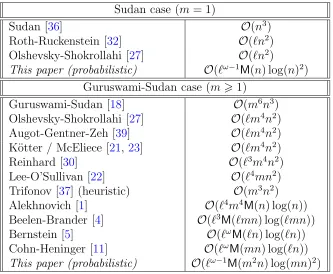
problem becomes known as a simultaneous Hermite-Pad´e approximation problem or vector Hermite-Pad´e approximation problem [3, 34]. The case µ= 1, with P1 being given through its roots (and their multiplicities) is known as the M-Pad´e problem [2]. Regarding Problem1, previous results focus on the Guruswami-Sudan cases = 1; we summarize them in Table3.1, in which we make assumptionsH1 andH2. In some
cases [30, 1, 5, 11], the complexity was not stated quite exactly in our terms but the translation is straightforward.
For this case, the most significant factor in the running time is its dependency with respect to n, with results either being cubic, quadratic, or quasi-linear. Then, under the assumption H1 : m 6 ℓ, the second most important parameter is ℓ, followed by
m. In particular, our result in Corollary 5compares favorably to the cost O˜(ℓωmn)
from [11], which was, to our knowledge, the best previous bound for this problem. In the general case s > 1, the result in Theorem 4 improves as well on the best previously known bounds; we discuss those below.
Sudan case (m= 1)
Sudan [36] O(n3) Roth-Ruckenstein [32] O(ℓn2) Olshevsky-Shokrollahi [27] O(ℓn2)
This paper (probabilistic) O(ℓω−1M(n) log(n)2) Guruswami-Sudan case (m>1)
Guruswami-Sudan [18] O(m6n3) Olshevsky-Shokrollahi [27] O(ℓm4n2) Augot-Gentner-Zeh [39] O(ℓm4n2) K¨otter / McEliece [21, 23] O(ℓm4n2) Reinhard [30] O(ℓ3m4n2) Lee-O’Sullivan [22] O(ℓ4mn2) Trifonov [37] (heuristic) O(m3n2) Alekhnovich [1] O(ℓ4m4M(n) log(n)) Beelen-Brander [4] O(ℓ3M(ℓmn) log(ℓmn)) Bernstein [5] O(ℓωM(ℓn) log(ℓn))
Cohn-Heninger [11] O(ℓωM(mn) log(ℓn)) This paper (probabilistic) O(ℓω−1M(m2n) log(mn)2)
Table 3.1: Overview of previous results, s= 1.
problem in terms of Gr¨obner basis computation in K[X, Y], implicitly or explicitly: the incremental algorithms of [21,26,23] are particular cases of the Buchberger-M¨oller algorithm [24], while Alekhnovich’s algorithm [1] is a divide-and-conquer change-of-order for bivariate ideals.
Yet another line of work [32, 39] uses Feng-Tzeng’s linear system solver [13], combined with a reformulation in terms of syndromes and key equations. We will use (and generalize to the case s > 1) some of these results in Section 3.5, but we will rely on the structured linear system solver of [7] in order to prove our main results. Prior to our work, Olshevsky and Shokrollahi also used structured linear algebra techniques [27], but it is unclear to us whether their encoding of the problem could lead to similar results as ours.
As said above, another approach rephrases the problem of computing Q in terms of polynomial matrix computations, that is, as linear algebra over K[X]; this was in particular the basis of the extensions to the multivariate casess >1 in [9,8]. Starting from generators of an ad-hoc K[X]-module (or polynomial lattice) that is known to contain a non-trivial Q, the algorithms in [22, 9, 4, 8, 5, 11] compute a Gr¨obner basis of that lattice, or simply a short vector therein. To achieve quasi-linear time in n (almost linear up to logarithmic factor), the algorithms in [4, 8] use a short vector subroutine due to Alekhnovich [1], while those in [5, 11] rely on a (faster, but probabilistic) algorithm due to Giorgi, Jeannerod and Villard [15]. For a lattice of dimensionL, with generators of degree at mostd, that algorithm in [4,8] runs in time O(LωM(d) log(Ld)). Note that a recent deterministic algorithm from [16] achieves the
same cost; this is the best result known to date.
Two main lattice constructions exist in the literature (Bernstein [5] gives more refined constructions, better adapted to some choices of the parameters). Follow-ing [9], we present them directly in the case s > 1; we give the cost bounds that can be obtained using the (fast) algorithms of [15,16] for lattice reduction. The first construction may be called banded (due to the shape of the generators it involves when s= 1); its generators derive from the polynomials Gand R introduced before:
(
Gi
s
Y
r=1
(Yr−Rr)jr
i >0, j1, . . . , js>0, i+|j|=m )
[ (Ys
r=1
(Yr−Rr)jrYrJr
j1, . . . , js>0, J1, . . . , Js>0, |j|=m, |J|6ℓ−m )
,
polynomials ( Gi s Y r=1
(Yr−Rr)jr
i >0, j1, . . . , js >0, i+|j|=m )
[ (Ys
r=1
(Yr−Rr)jr
j1, . . . , js >0, m6|j|6ℓ )
.
When s = 1, the first construction is used in [4, Remark 16] and [22, 11] and the second is used in [4, 5]; the latter also appears in [8] for s > 1. In both cases, the actual lattice bases are the coefficient vectors (in Y) of the polynomials
h(X, XkY
1, . . . , XkYs), forh in either of the sets above.
For the banded basis, we have the following dimension and degree bounds, from [9]:
Lb =
s+m−1
s
+
s+m−1
s−1
s+ℓ−m s
and db =O(mn);
in the triangular case, we have
Lt =
s+ℓ s
and dt=O(ℓn).
Under our assumption m 6 ℓ, we always have Lb >Lt and db 6 dt; when s = 1, we
getLb =Lt =ℓ+ 1. In both cases, we readily deduce the cost of finding a polynomial
Q from [15,16], respectively to O(Lω
bM(db) log(Lbdb)) and O(LωtM(dt) log(Ltdt)).
For s = 1, these are the costs reported in [5, 11]. For s > 1, the costs reported in [9, 8] are worse, because the short vector algorithms used in thoses references are inferior to the ones we refer to. UnderH1 andH2, and possibly neglecting logarithmic
factors from O notation, the result in Theorem 4 is an improvement over those of both [9] and [8]. To see this, remark that the cost in our theorem is quasi-linear in
s+ℓ s
ω−1 s+m
s+1
n, whereas the costs in [9,8] are at least s+sℓωmn; a quick simplification proves our claim.
weighted-degree condition, the following condition must hold:
deg(det(L)) dimL < b.
For both lattices described above, assuming as beforem6ℓ, one can verify that this inequality can be rewritten
1
s+ℓ s
X
06|i|<m
n(m− |i|) + X 06|j|6ℓ
|j|k
< b.
This is precisely the assumption M < N seen before.
Outline of the paper. The next section briefly discusses the relevance of assump-tionH1. Then, after a reminder on algorithms for structured linear systems, we show
how to reduce Problem 1 to Problem2 in Section 3.4, then give two algorithms that both prove Theorem 3, in Sections3.5 and 3.6.
3.2
Preliminaries: assumption H1
In this very brief section, we discuss assumption H1 that was introduced previously for Problem 1. In Theorem 4, we do not make any assumption on m and ℓ, but we mentioned that assumption H1, that is, m 6 ℓ is mostly harmless. The following
lemma substantiates this claim, by showing that the case m > ℓ can be reduced to the case m = ℓ. As mentioned in the introduction, we denote by G the master polynomial Q16i6n(X−xi).
Lemma 6. Suppose that m >ℓ. Then, if b < n(m−ℓ), Problem 1 with parameters
(s, ℓ, m, n, k, b) has no solution. Else, the solutions to that problem are exactly the
polynomials of the form Q = Q⋆ Gm−ℓ, where Q⋆ is a solution to Problem 1 with
parameters (s, ℓ, ℓ, n, k, b−n(m−ℓ)).
Proof. Let Q be a solution to Problem 1 with parameters (s, ℓ, m, n, k, b). We claim that b > n(m−ℓ), that Gm−ℓ divides Q, and that Q⋆ = Q/Gm−ℓ is a solution to
Problem 1with parameters (s, ℓ, ℓ, n, k, b−(m−ℓ)).
Let i be in {1, . . . , n}. By condition (iv), Qi = Q(X+xi, Y1+yi,1, . . . , Ys+yi,s)
has no monomial of total degree less than m. By condition (ii), every monomial in
Qi has degree at most ℓ inY, so each such monomial is a multiple ofXm−ℓ. Shifting
Let then Q⋆ =Q/Gm−ℓ. This polynomial is nonzero, has degree at most ℓ inY, and
Q⋆(X, XkY1, . . . , XkYs) =Q(X, XkY1, . . . , XkYs)/Gm−ℓ.
Since the numerator on the right-hand side has degree less than b, and Q⋆ is nonzero
we must in particular have b > n(m−ℓ), as claimed. Besides, for 1 6 i 6 n, the remarks above show that Q⋆(x
i, yi,1, . . . , yi,s) = 0 with multiplicity ℓ. Thus, Q⋆ is a
solution to Problem 1 with parameters (s, ℓ, ℓ, n, k, b−n(m−ℓ)).
Conversely, let Q′ be any solution to Problem 1 with parameters (s, ℓ, ℓ, n, k, b−
n(m−ℓ)). Proceeding as in the previous paragraphs, one easily verifies thatQ′ Gm−ℓ
is a solution to the problem with parameters (s, ℓ, m, n, k, b), so the proof is complete.
3.3
Solving structured linear systems
Our main algorithms rely on solving linear systems overK. In this section, we briefly review useful concepts and results related to displacement rank techniques. While these techniques can handle systems with several kinds of structure, we will only need (and discuss) those related to Toeplitz-like and Hankel-like systems (explained in chapter 2); for a more comprehensive treatment, the reader may consult [28].
Let M be a positive integer and let ZM ∈KM×M be the square matrix with ones
on the subdiagonal and zeros elsewhere:
ZM =
0 0 · · · 0 0 1 0 · · · 0 0 0 1 0 · · · 0
..
. . .. ... ... ... 0 · · · 0 1 0
∈KM×M.
Given two integers M, N, consider the following operators: ∆M,N : KM×N → KM×N
A 7→ A− ZM AZNT
and
∆′
M,N : KM×N → KM×N
which subtract from A its translate one place along the diagonal, resp. along the anti-diagonal.
Let us discuss ∆M,N first. If A is a Toeplitz matrix, that is, invariant along
diagonals, ∆M,N(A) has rank at most two. As it turns out, Toeplitz systems can
be solved much faster than general linear systems, in quasi-linear time in M. The main idea behind algorithms for structured matrices is to extend these algorithmic properties to those matrices Afor which the rank of ∆M,N(A) is small, in which case
we call A Toeplitz-like. Below, this rank will be called the displacement rank of A
(with respect to ∆M,N).
Two matrices (V, W) in KM×α×Kα×N will be called agenerator of length αforA with respect to ∆M,N if ∆M,N(A) =V W. For the structure we are considering, one
can recover A from its generators; in particular, one can use a generator of length α
as a way to represent A using α(M +N) field elements. One of the main aspects of structured linear algebra algorithms is to use generators as a compact data structure throughout the whole process.
Up to now, we only discussed the Toeplitz structure. Hankel-likematrices are those which have a small displacement rank with respect to ∆′
M,N, that is, those matrices
A for which the rank of ∆′
M,N(A) is small. As far as solving the system Au = 0 is
concerned, this case can be easily reduced to the Toeplitz-like case. DefineB =AJN,
where JN is the reversal matrix of size N, all entries of which are zero, except the
anti-diagonal which is set to one. Then, one easily checks that the displacement rank of Awith respect to ∆′
M,N is the same as the displacement rank ofB with respect to
∆M,N, and that if (V, W) is a generator for A with respect to ∆′M,N, (V, W JN) is a
generator forB with respect to ∆M,N. Using the algorithm for Toeplitz-like matrices
gives us a solution v to Bv= 0, from which we deduce that u=JNv is a solution to
Au= 0.
In this paper, we will not enter the details of algorithms for solving such structured systems. The main result we will rely on is the following proposition, a minor exten-sion of a result by Bostan, Jeannerod and Schost [7], which features the best known complexity for this kind of task, to the best of our knowledge. This algorithm is based on previous work of Bitmead-Anderson [6], Morf [25], Kaltofen [20] and Pan [28], and is probabilistic (it depends on the choice of some parameters in the base field, and suc-cess is ensured provided these parameters avoid a strict hypersurface of the parameter space).
re-duce the cost so that it only depends on M, not max(M, N)), but that would be inconsequential for the applications we make of it.
Proposition 7. Given a generator (V, W) of length α for a matrix A ∈ KM×N,
with respect to either ∆M,N or ∆′M,N, one can find a non-zero element in the
nullspace of A, or determine that none exists, by a probabilistic algorithm that uses
O(αω−1M(P) log(P)2) operations in K, withP = max(M, N).
The algorithm choosesO(P)elements inK; if these elements are chosen uniformly
at random from a set S ⊂ K of cardinality at least 6P2, the probability of success is
at least 1/2.
Square matrices. In all that follows, we consider only the operator ∆M,N, since
we already pointed out that the case of ∆′
M,N can be reduced to it at no extra cost.
When M = N, we use directly [7, Theorem 1], which gives the running time reported above. That result does not explicitly state which solution we obtain, as it is written for general non-homogeneous systems. Here, we want to make sure we obtain a nonzero nullspace element (if one exists), so slightly more details are needed. The algorithm in that theorem chooses 3M −2 elements in K, the first 2M −2 of which are used to precondition A by giving it generic rank profile; this is the case when these parameters avoid a hypersurface of K2M−2 of degree at most M2+M.
Assume this is the case. Then, the output vector u is obtained in a parametric form as u=ℓ(u′), where u′ consists of another set ofM parameters chosen in K and
ℓ is a surjective linear mapping with image the nullspace ker(A) of A. If ker(A) is trivial, the algorithm returns the zero vector in any case, which is correct. Otherwise, the set of vectors u′ such that ℓ(u′) = 0 is contained in a hyperplane of KM, so it is
enough to choose u′ outside of that hyperplane to ensure success.
Using the Zippel-Schwartz lemma and the obvious upper bound M2 +M + 1 6 3M2, we conclude that if we choose all parameters uniformly at random in a subset
S of K of cardinality at least 6M2, the algorithm succeeds with probability at least 1/2.
Tall matrices. Suppose finally that M > N. This time, we build the matrix
A′ ∈ KM×M by adjoining M − N zero columns to A on the left. The generator
(V, W) of A can be turned into a generator of A′ by simply adjoining M −N zero columns to W on the left. We then solve the system A′s= 0, and return the vector
u obtained by discarding the first M −N entries of s.
The cost of this algorithm fits into the requested bound; all that remains to see is that we obtain a nonzero vector in the nullspace ker(A) of A with nonzero probability. Indeed, the nullspaces of A and A′ are now related by the equality ker(A′) =KM−N×ker(A). We mentioned earlier that in the algorithm for the square
case, the solution s to A′s = 0 is obtained in parametric form, as s = ℓ(s′) for
s′ ∈KM, with ℓ a surjective mappingKM →ker(A′). Composing with the projection
π : ker(A′) →ker(A), we obtain a parametrization of ker(A) as u = (π◦ℓ)(s′). The error probability analysis is then the same as in the square case.
3.4
Reducing Problem
1
to Problem
2
In this section, we show how instances of Problem 1 can be reduced to instances of Problem 2. The main technical ingredient, stated in Lemma 8 below, generalizes to any s > 1 the one given for s = 1 by Zeh, Gentner, and Augot in [39, Proposition 3]. To prove it, we use the same steps as in [39]; we rely on the notion of Hasse derivatives, which allow us to write Taylor expansions in positive characteristic (see for instance Hasse [19] or Roth [31, pp. 87, 276]).
In what follows, comparison and addition of s-tuples of integers are defined com-ponentwise. For example, writing i 6 j is equivalent to ik 6 jk for k = 1, . . . , s,
and i−j denotes (i1−j1, . . . , is−js). Similarly, ify= (y1, . . . , ys) is in K[X]s then
Y −y= Y1−y1, . . . , Ys−ys. Finally, for products of binomial coefficients, we shall
write
j i
=
j1
i1
· · ·
js
is
.
Note that this coefficient is zero when i 66 j; note also that the monomial Yi has
total degree degY(Yi) =|i|=i1+· · ·+is.
IfAis any commutative ring with unity andA[Y] denotes the ring of polynomials in Y1, . . . , Ys over A, then for a polynomial P(Y) = PjPjY
j in A[Y] and a