Argentina: Feeding on food crisis?

Argentina: Feeding on Food Crisis?

Ahmet Ozyigit (Middlesex University,United Kingdom)

Fehiman Eminer (Department of Economics, Near East University, Nicosia, Cyprus)

†

© 2011 Asian Economic and Social Society. All rights reserved ISSN(P): 2309-8295 ISSN(E): 2225-4226

www.aessweb.com Author(s)

Ahmet Ozyigit †

Middlesex University, United Kingdom Email: aozyigit@neu.edu.tr

Fehiman Eminer

Department of Economics, Near East University, Nicosia, Cyprus

Argentina: Feeding on Food Crisis?

Abstract

This article uses a Vector Error Correction Model (VECM) framework to estimate simultaneously the short-run and long-run relationship between food price inflation and poverty reduction in Argentina. Results from the cointegration tests reveal that economic growth, food price inflation and poverty reduction exhibit a long-run relationship. The results from the VECM support the argument that there exists a uni-directional causality running from food price inflation and economic growth to poverty reduction, but not the other way around. Argentina has, in fact, witnessed substantial poverty reduction as a response to the global food crisis by maintaining its position as a net exporter of food products.

Keywords: Argentina, food price inflation, global food crisis, cointegration, vector error correction, agriculture-led growth, poverty reduction

Introduction

inflation as early as 2002. With more than two billion people worldwide living on less than $2 a day and another 880 million living on less than $1 a day, increase in food prices has had devastating effects throughout the world (World Development Report, 2008).

A change in the price of a commodity can be explained as a response to a change in demand or a change in supply. On the demand side, increasing food prices is attributed to the growth of world population. As more people exist, there is necessarily an upward pressure in the demand for food. Aside from increases in population, researchers also list growing meat consumption as a reason for the upward trend in global food crisis as it stimulates demand for animal feed (Benson et. al., 2008). On the supply side, a number of factors have been associated with increasing global food crisis. Recent draughts, increased concerns over the demand for bio-fuel production and decreased supply of labor employed in the agricultural sector have been identified as the main supply factors of food price inflation.

Despite the general consensus on the devastating effects of increasing food prices all over the world, not every economy is affected by increased food prices by the same magnitude. U.N. Secretary-General Ban Ki-moon called the food crisis the “crisis for the most vulnerable”, as it is the poorest that spend a greater share of their income on food. Therefore, those economies with larger poverty gaps and headcount are likely to be struck by increased food prices more that those that are economically better off. However, poverty is not the only measure of scale

with which increased food prices affect the economy of a nation. The ability to produce and possibly sell food products abroad will also determine the rate at which food prices affect the local economy. As the net importers of food will be forced to pay higher amounts for their imports, the net exporters will in fact enjoy better terms of trade and benefit from increased food prices in terms of higher export revenue. One such case is the case of Argentina. As a net exporter of food products, Argentina stands out from the rest of the South American countries in its experience with food price inflation. This is evidenced by the following table where in majority of the South American economies, the food price inflation by far exceeds the overall level of inflation while in Argentina this does not seem to be the case.

Figure 1: Food and overall inflation in South America, 2007

2

Source: National statistical institutes, adopted from FAO (2008)

Perhaps one of the main reasons why Argentina stands out in the region has something to do with the food production and exporting capabilities. “Argentina’s agricultural sector … represents 7 percent of its GDP and provides jobs for 12 percent of the labor force. However, Argentina depends heavily on agriculture for export earnings-52 percent of merchandise export value comes

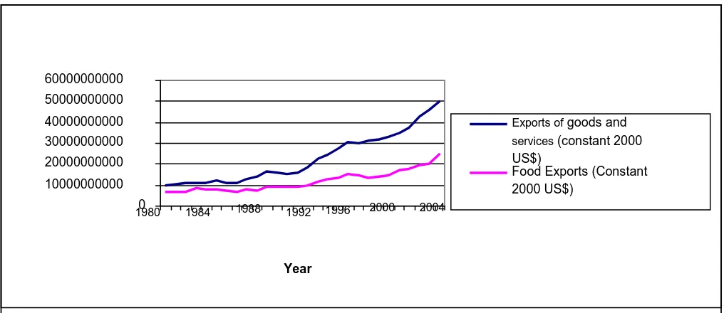
from agricultural products” (USDA, 2001). This dependence is not necessarily bad for the Argentinean economy as it has enabled higher export revenues in the face of increasing food prices. To have a better idea of Argentina’s exporting behavior we shall look at the figure below which shows a time series of the overall volume of exports and food exports:

Figure 2: Argentinean exports (1980-2000) at constant 2000 US$

Source: World Bank, World Development Indicators Online (2009)

The increasing trend of exporting activity, especially accelerating after 2002, is coupled with the food price inflation that takes off around the same time (as evidenced by figure 3 below). This increase in food exports along with the price of food products necessarily benefits the Argentinean economy through improved terms of trade and higher export earnings.

There exist numerous studies analyzing the relationship between agricultural growth and economic growth as well as poverty reduction. One could identify this notion as agriculture-led growth as a means to eliminate poverty and income inequality. Peter Timmer uses the Deininger-Squire data set for poverty and purchasing power for 35 developing countries and finds that "a one percent growth in agricultural GDP per capita leads to a 1.61 percent increase in per capita incomes of the bottom quintile of the population" (Timmer, 1997). Preceding studies of Ravallion and Datt (1996),Ahluwalia (1978), and Mellor and Desai (1985) also show strong evidence for the poverty reduction aspect of an increase in agricultural GDP. Furthermore, the report of Inter-American Development Bank fits almost a perfect line to the positive relationship between agricultural growth of value

added and economic growth in the entire Latin American region between 1990 and 1997 (IADB, 1997).

Figure 3: Food price index (Base year, April 2008

Source: INDEC (2009)

In Argentina, apart from food production and agricultural growth, food price inflation has also enabled improved

Index = 100

0 2 0 4 0 6 0 8 0 10 0 12 0

199 5

199 6

199 7

199 8

199 9

200 0

200 1

200 2

200 3

200 4

200 5

200 6

200 7

200 8

200 9 Food Price Index 0

10000000000 20000000000 30000000000 40000000000 50000000000 60000000000

1980 1984 1988 1992 1996 2000 2004

Year

Exports of goods and

services (constant 2000 US$)

3 terms of trade and in fact contributed to the local economy both in terms of increased export revenues, economic growth and poverty reduction. This is evidenced by the strong negative trending relationship between food prices and headcount poverty rates as shown in figure 4 below:

Figure 4: Poverty headcount ratio vs. food price inflation

Note: Poverty Headcount corresponds to the percentage of households below the poverty line. Food price index uses 2008 as the base year.

Source: INDEC (2009)

The aim of this article is to reveal any possible long run relationships between food prices, poverty and per capita growth in Argentina. For this end, a cointegration relationship is established in an error correction framework. The rest of the article is structured as follows: Part II introduces the data and methodology. Part III presents the empirical results and interpretations and finally part IV concludes with possible policy recommendations.

Data and methodology

Data used in this article is pooled from the National Institute of Statistics and Census of Argentina (INDEC) and the Economic Commission for the Latin America and the Caribbean (ECLAC). Data includes semi-annual series of food price index (FP), Poverty (P) as measured by the headcount ratio, and GDP (Y) in 1993 millions of Pesos between 1988 and the first half of 2009. All the variables are in their regular forms as opposed to logarithms since variables are either provided as indices or in small scales. As a result, there is no need to compress the scale further by taking the logarithms, trend and a dummy variable for the year 2002 where food

prices begin to soar. The first step of analysis is to investigate the integration properties of the series. For this end, the modified Dickey and Fuller (1979) test proposed by Elliott et al. (1996) is administered. Perron and Ng (1994) have shown that the DF-GLS has better finite-sample properties than the conventional Dickey-Fuller and Phillips-Perron tests. Once the integration properties of the data are checked for, we move on to determine the long run relationship properties between GDP, Poverty headcount and food prices. For this end, this paper implements the Johansen and Juselius (1990) and

Johansen (1991) cointegration procedure. The

cointegration test is based on the following vector error correction model (VECM):

p

∆Yt= δ0+ ∑ δi∆Yt-i + α β’ Yt-p + μt ..………. (1)

i=1

Where ∆ is the difference operator, Yt is the 3x1 vector of the endogenous variables (Y, FP and P), δ represents the intercept and μ represents the vector of the white noise process. The matrix β consists of the cointegration vectors, whose number will be revealed by the trace and the maximum eigenvalue statistics following the Johansen and Juselius cointegration procedure. In order to account for the short-run and long-run dynamics between the variables, the following VECM is formulated:

ΔY =δ1+lagged (ΔY, ΔP, ΔPF)+ α1EC(−1) …..(2) ΔP =δ2+lagged (ΔY, ΔP, ΔPF)+ α1EC(−1) …..(3) ΔPF =δ3+lagged (ΔY, ΔP, ΔPF)+ α1EC(−1) …..(4)

where EC(-1) is the error correction term lagged by one period. The error correction term identifies the deviations of the series from the long-run equilibrium. Significance of the error correction term in the VECM equations leads us to reject the null hypothesis of non-causality among the variables in the long-run. The first two equations might yield significant results for long run causality; however, a significant finding in equation 4 will not entirely make sense as food prices are not expected to be tied to GDP or the headcount poverty rates.

Results and interpretation

The time series properties of the series are examined first by applying the DF-GLS (DF for short) and PP unit root tests. Table 1 below presents the unit root test statistics obtained from both testing methods:

Figure 4: Poverty Headcount Ratio vs. Food Price Inflation

4 Table 1: DF-GLS and PP tests for unit root

Statistics (Level) Y Lag FP Lag P lag

τT (DF) -2.52 2 -1.04 0 -1.60 1

τμ (DF) -1.06 2 -0.20 0 -1.68 1

τ (DF) 2.53 0 3.40 0 -0.98 1

τT (PP) -1.43 2 -1.51 3 -1.67 3

τμ (PP) 0.68 1 -0.43 3 -1.75 3

τ (PP) 2.50 1 2.24 3 -0.93 2

Statistics (First Difference) ∆ Y Lag ∆ FP Lag ∆ P lag

τT (DF) -3.20*** 2 -3.80** 0 -5.49* 0

τμ (DF) -3.23** 2 -3.87* 0 -4.80* 0

τ (DF) -2.36** 1 -3.08* 0 -4.38* 0

τT (PP) -6.10* 1 -3.80** 1 -5.70* 1

τμ (PP) -5.94* 1 -3.87* 1 -5.73* 1

τ (PP) -5.43* 2 -3.08* 0 -5.77* 1

Note: τT represents the most general model with a drift and trend; τμ is the model with a drift and without trend; τ is the most restricted model without a drift and trend. Numbers in brackets are lag lengths used in DF test to remove serial correlation in the residuals. When using PP test, numbers in brackets represent Newey-West Bandwith (as determined by Bartlett-Kernel). Both in DF and PP tests, unit root tests were performed from the most general to the least specific model by eliminating trend and intercept across the models (See Enders, 1995: 254-255). *, ** and *** denote rejection of the null hypothesis at the 1% , 5% and 10% levels respectively. Tests for unit roots have been carried out in E-VIEWS 6.0

Both DF-GLS and PP unit root tests fail to reject the null hypothesis of the existence of a unit root in all of the series at the levels. However, when the series are first differenced, both DF-GLS and PP statistics reject the null hypothesis of a unit root. Therefore, both test results agree that the series are stationary in their first differences, meaning all of the

variables used in our analysis are integrated of order one (I(1)). The decision about the lag length of the model is based on the Akaike Information Criterion, AIC, Schwarz Criterion, SC and Hannan–Quinn Criterion, HQC. Based on these criteria, the lag order is selected to be 3 as shown by the table below.

Table 2: Lag length selection criteria

Lag LogL LR FPE AIC SC HQ

0 18.103 NA 0.000104 -0.654 -0.393 -0.562

1 146.815 222.635 1.62e-07 -7.125 -6.472 -6.894

2 193.485 73.1584 2.15e-08 -9.161 -8.116 -8.792

3 225.628 45.174* 6.38e-09* -10.412* -8.975* -9.905*

4 234.826 11.435 6.72e-09 -10.303 -8.594 -9.778

5 245.584 11.630 6.78e-09 -10.218 -8.297 -9.735

6 253.355 7.140 8.54e-09 -9.451 -7.839 -9.530

Note: Maximum Lag of 6 is selected to avoid under estimation of the lag length

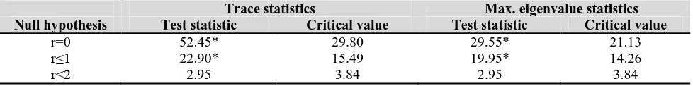
As all of the criteria presented in this table agree with the lag length of 3, we specify the lag length to be 3. Next, we need to determine whether the I (1) variables are cointegrated using the Johansen multivariate

cointegration process. Both the trace and the maximum eigenvalue test statistics of cointegration are provided by the table below:

Table 4: Johansen multivariate cointegration test results

Trace statistics Max. eigenvalue statistics

Null hypothesis Test statistic Critical value Test statistic Critical value

r=0 52.45* 29.80 29.55* 21.13

r≤1 22.90* 15.49 19.95* 14.26

r≤2 2.95 3.84 2.95 3.84

Note: * indicates rejection of the null hypothesis at the 5% level. Test Statistics are obtained from the E-views 6.0 software

Before estimating the VECM, one last step is applying the weak exogeneity test on the variables to measure the long-run relationship in the cointegrating vector. The

5 can suggest that short-run innovations in variables in fact have long-run implications. Table 5 below reports these

test statistics:

Table 5: LR test for weak exogeneity

r DGF Y FP P

1 2

1 2

20.68* 5.21*

20.74* 6.33*

19.33* 1.81

Notes: r stands for the number of cointegration ranks. DGF stands for degrees of freedom. * denotes significance at the 5% level

Rejection of weak exogeneity for most of the variables in the system suggests that the variables are endogenous, meaning, short term innovations are likely to have long term impacts. For instance, with r =1, we reject weak exogeneity for all of the variables in the system. Hence,

we are ready to employ VECM approach as we are convinced that the series are cointegrated and a long run relationship exists between them. Table 6 below summarizes the VECM estimates:

Table 6a: VECM Estimates for ΔY equation

Coefficient Std. Error t-Statistic Prob.

C 2.653 2.904 0.913 0.369

D(Y(-1)) 0.137 0.180 0.7598 0.453

D(Y(-2)) 0.363 0.216 1.677 0.105

D(Y(-3)) -0.135 0.209 -0.644 0.524

D(FP(-1)) 0.635 0.559 1.135 0.266

D(FP(-2)) -0.413 0.612 -0.674 0.505

D(FP(-3)) -0.329 0.602 -0.546 0.589

D(P(-1)) -0.522 0.536 -0.973 0.339

D(P(-2)) 0.378 0.487 0.777 0.443

D(P(-3)) -0.068 0.450 -0.153 0.879

D2002 7.883 12.771 0.617 0.542

EC(-1) 0.490 0.218 2.239* 0.033

Note: * denotes significance at 5%

With the significant t-statistic at 5% for the error correction term, we can confidently argue that poverty headcount and the food prices Granger-cause GDP in the long-run. However, none of the coefficients are

significant, suggesting no short-run causality. Table 6b below analyzes the short run and the long run dynamics of the ΔPF equation:

Table 6b: VECM Estimates for ΔFP equation

Coefficient Std. Error t-Statistic Prob.

C 0.795 0.858 0.926 0.362

D(Y(-1)) -0.052 0.053 -0.989 0.331

D(Y(-2)) -0.019 0.064 -0.311 0.757

D(Y(-3)) 0.031 0.061 0.515 0.610

D(FP(-1)) 0.475 0.165 2.878* 0.007

D(FP(-2)) 0.154 0.181 0.855 0.400

D(FP(-3)) 0.037 0.178 0.209 0.835

D(P(-1)) -0.039 0.158 -0.247 0.806

D(P(-2)) -0.124 0.144 -0.862 0.396

D(P(-3)) 0.083 0.133 0.630 0.533

D2002 13.956 3.774 3.697* 0.001

EC(-1) -0.075 0.064 -1.174 0.250

Note: * denotes significance at 5%

The evidence provided by this table is completely in line with the opening arguments of this article. The error correction term is not significant, suggesting that GDP

6 run, food prices are Granger-caused only by its lagged term. The significant and substantially high coefficient for the dummy variable placed for the take off of food price inflation in 2002 also suggests a significant turning point in food prices. Finally, and most importantly, we shall turn to the long-run causal effect of GDP and food

prices on the rate of poverty. As suggested in previous parts of this article, we expect to see a negative relationship between food price inflation, GDP growth and poverty rates. Table 6c below summarizes the findings:

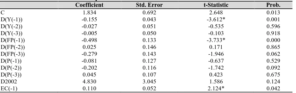
Table 6c: VECM Estimates for ΔP equation

Coefficient Std. Error t-Statistic Prob.

C 1.834 0.692 2.648 0.013

D(Y(-1)) -0.155 0.043 -3.612* 0.001

D(Y(-2)) -0.027 0.051 -0.535 0.596

D(Y(-3)) -0.005 0.050 -0.103 0.918

D(FP(-1)) -0.498 0.133 -3.733* 0.000

D(FP(-2)) 0.025 0.146 0.171 0.865

D(FP(-3)) -0.279 0.143 -1.946 0.062

D(P(-1)) -0.081 0.127 -0.637 0.529

D(P(-2)) -0.202 0.116 -1.742 0.092

D(P(-3)) 0.045 0.107 0.423 0.675

D2002 4.830 3.045 1.586 0.124

EC(-1) 0.110 0.052 2.124* 0.042

Note: * denotes significance at 5%

Conforming to the arguments made throughout the article, we see that GDP with one lag Granger-causes poverty reduction (as evidenced by the significant negative coefficient). The same is true for food prices. The significant negative coefficient (even higher than the GDP coefficient) implies that there is a short run Grange causality running from food prices to poverty reduction. Finally, the significant error correction term suggests that GDP and Food Prices both Granger-cause Poverty reduction in the long run.

Conclusion

This study presents empirical evidence for the provocative and against-the –literature suggestion that food price inflation has in fact benefited the Argentinean economy and resulted in poverty reduction. Our

empirical findings suggest that increasing food prices in fat do more in terms of poverty reduction compared to GDP growth. As a net exporter of agricultural products, Argentina has enjoyed improved terms of trade with respect to agricultural product exports and enjoyed higher gains from trade. This has also reflected upon the Argentinean population in terms of poverty reduction.

These results should be treated with caution, however. Even though global increase in the food prices has been somewhat higher than the Argentinean food prices (as evidenced by figure 1), further growth and further reduction in poverty may not be sustainable only by this increase in prices. As a net exporter of food products, Argentina not only needs to maintain its position as a net exporter but also develop alternative strategies in the case of a future decline in world food prices.

Views and opinions expressed in this study are the views and opinions of the authors, Journal of Asian Business Strategy shall not be responsible or answerable for any loss, damage or liability etc. caused in relation to/arising out of the use of the content.

References

Ahluwalia, M. S. (1978). Rural poverty and agricultural performance in India. Journal of Development Studies, 14, 298-323.

Benson, T., Minot, N., Pender, J., Robles, M. Y., & Braun, J. (2008). Global food crisis. Monitoring and Assessing Impact to Inform Policy Responses. IFPRI (September, 2008).

http://www.ifpri.org/pubs/fpr/pr19.pdf.

Dickey, D., & Fuller, W. (1981). Likelihood Ratio Statistics for Auto Regressive Time Series with a Unit Root. Econometrica, 49(4), 39-45.

Elliott, G., Rothenberg, T., & Stock, J. (1996). Efficient test for an autoregressive unit root. Econometrica, 64(6), 813-836.

7 over-action needed. Newsroom. June 3, 2008. Rome, Italy: FAO.

<http://www.fao.org/newsroom/en/news/2008/100 0853/index.html>

Inter-American Development Bank (IADB), Statistical Report, (1997).

Argentinean National Institute for Statistics and Censuses (INDEC), Statistical Database, (2009).

Johansen, S. (1991). Estimation and hypothesis testing of cointegration vectors in Gaus-Sian vector autoregressive models. Econometrica, 59, 1551-1580.

Johansen, S., & Juselius, K. (1990). Maximum likelihood estimation and inferences on cointegration with applications to the demand for money. Oxford Bulletin of Economics and Statistics, 69, 675-684. Mellor, J., & Desai, G. (eds) (1985). Agricultural change

and rural poverty. Baltimore: Johns Hopkins University Press.

Ravallion, M., & Datt, G. (1996). How Important to India’s Poor is the Sectoral Composition of Economic Growth. The World Bank Economic Review, 10, 1.

Perron, P., & Ng, S. (1994). Useful modification to some unit root tests with dependent errors and their asymptotic properties. Department de Sciences Économiques, Montreal, PQ: Universite de Montreal.

Timmer, C. P. (1997). How well do the poor connect to the growth process. CAER Discussion Paper No. 178. Harvard institute for international development (HIID), Cambridge, MA.

United States Department of Agriculture (2001). Economic research service. Agriculture in Brazil

and Argentina.

http://www.ers.usda.gov/publications/wrs013/wrs0 13c.pdf.

World Bank (2008). rising global prices: The World

Bank’s latin American and caribbean region

position paper. First Draft for Discussion March 24, 2008. Washington, DC, United States: World Bank.