Bayes Interval Estimation for binomial proportion and difference of
two binomial proportions with Simulation Study
1
Masoud Ganji
,Solmaz Aghlmandi
21
Department of Statistics , Faculty Mathematical Science , University of Mohaghegh Ardabili
Ardabil , Iran
2
Department of Statistics , Faculty Mathematical Science , University of Mohaghegh Ardabili
Ardabil , Iran
Abstract
This study is considered a number of popular confidence interval for binomial proportion and the difference of two binomial proportions . A new approach is proposed base on Bayesian view for binomial proportion and also for difference of two binomial proportions . The Bayes confidence intervals compared with other confidence intervals of coverage probability and expected length . Based on this analysisand t he simulation study recommend the , Bayes confidence interval of binomial proportion and difference of two binomial proportions for small sample , and show their superior performance from both criteria .
Keywords: Bayes interval, coverage proba- bility, confidence interval, expected lengths.
1. Introduction
In recent years the interval estimation of binomial proportion and difference of two binomial proportions has been reviewed. This is due to poor and irregular behavior of Wald confidence interval of coverage probability , it is mentioned by Agresti and Coull[1] , Agresti and Caffo[2], Brown et al.[5] and Newcomb[7] . Standard confidence interval is used globally , since it’s structure is simple , and it can be accounted as the representative of confidence interval for binomial proportion and difference
much confidence interval (CI) such as Wilson CI , arcsine CI , logit CI , exact CI , likelihood ratio CI and Jefferys CI for binomial prop- ortion. It should explained that , the Bayes estimator 0.5
1
x p
m
+ =
+
is obtained by using the
Jeffery Beta form , with parameters (0.5,0.5) as a prior distribution , and the Jeffery approximate CI obtained by using the normal approximation . For such estimator, this CI , is recommended for small sample size (less than 40) (Brown et al.[5], [6]) .
There for , we apply the Beta( , )α β prior distribution and normal approximation to make Bayes approximate CI . We know that , the prior distribution Beta( , )α β for binomial distribution
is conjugate . If we assume that X ~binom n p( , )
, and p has the prior distribution Beta( , )α β , the posterior distribution of p is Beta x( +α,m− +x β).
By using of the normal approximate , we get :
(1 )
| ~ ( , )
( 1)
p p
P x N p
n α β
− + + +
(1)
There for by notice to the above approximation , we can proposed the Bayes approximate of CI and in section 2 and 3 we show that , for suitable amount of
α
and β in comparison with the other CIs , the Bayes CI involve the best performance in the coverage probability and expected length .2. Confidence interval of binomial
proportion and difference of two
binomial proportions
2.1. Confidence interval of binomial
proportion
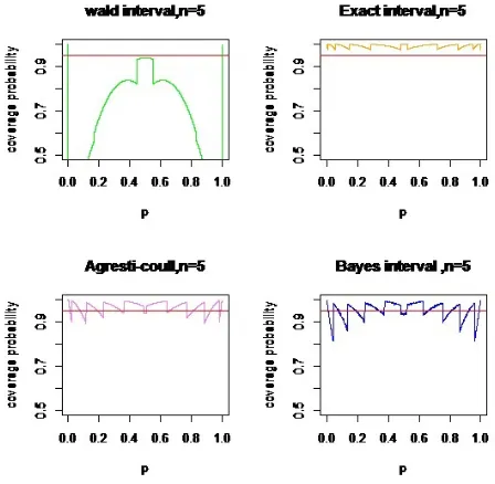
Fig. 1 coverage probability of 95% confidence intervals for n=5
Wald CI (
CI
w ): Ifx x
1,
2,.,
x
nis a random sample from binomial distribution with unknown parameter P and known parameter n ,the MLE of p is pˆ x
n
= . As it is mentioned in
most of text books CIw of p is equal with :
2
ˆ ˆ(1 ˆ) /
w
CI = ±p zα p − p n (2)
Where
z
α/ 2denote the upperα
/ 2
quintile of the standard normal distribution.Agresti-Coull CI (
CI
A C ) : Agresti and Coull[1] improved CIw , by adding two successes and twofailures to the sample size , that is , they replaced
n by n= +n 4 and pˆ with 2
4
x p
n
+ =
+
, which is
performance improved the CIw. The CIA Cis as :
2
(1 ) / A C
CI = ±p zα p − p n (3)
Exact CI (
CI
E): In contrast to CIw , mostCIEwhich presented by Clopper-Pears on (1934) .
CIEof p , obtained by inverting the binomial test of H0 : p p= 0 with equal-taild and by solving the following equations with respect to p0 , i.e :
0 0
0
(1 ) 2 x
k n k
k
p p
n k
α −
=
− =
∑
and
0 (1 0) 2 n
k n k
k x
p p
n k
α −
=
− =
∑
This estimated CIEensures that , coverage probability for all of the amount of p is at least 1−α , for x=1,2,...n-1 . The CIE is as follows :
1
2 ,2( 1),1 /2
1
[1 ]
E
x n x
n x
CI p
xF α
−
− + − − +
= + < (4)
Where Fa b c, , is measure of F distribution with "a" and "b" degree of freedom and "1-c" quintile .
Fig. 2 coverage probability of 95% confidence intervals for n=50
Bayes CI (
CI
B ): According to prior distribution Beta(2 , 2 ) , the posterior of p is :| ~ ( 2, x 2)
P x Beta x + n− +
By using the normal approximate we get:
(1 )
| ~ ( , )
( 5)
p p
P x N p n
− +
and by using 2 4
x p
n + =
+
as a estimation of p ,
CIBcan be obtained as follows :
2
(1 ) / ( 5)
B
CI = ±p zα p −p n+ (5)
Fig. 3 average expected lengths of 95% confidence intervals, n=15
2.2. Confidence interval of difference of two
binomial proportions
The following notation used frequently in this article.
1 ( , )
X binom n p , y binom n p( , 2), ∆ =p1−p2 , 1
i i
q = −p , i=1 , 2 and the MLE of p1and p2are
1 ˆ X
p n
= ,
2
ˆ y
p m
= respectively.
Wald CI (CIW* ) : The distribution of statistics
ˆ ˆ
( )
T σ∆
∆ − ∆
= approximately tends to the standard
normal distribution , since σ∆ˆ is the consistent estimator of V ar( )∆ =p q1 1/n+p q2 2/m , we can replace MLE of the parameters in above formula
1 2( 1),2( ), /2
[1 ]
( 1) x n x
n x
x F α
−
+ −
− < +
i.e . V ar( )∆ =ˆ p qˆ ˆ1 1/n+p qˆ ˆ2 2/m , where
1 2 ˆ pˆ pˆ
∆ = −
and get CI* Was;
*
1 1 2 2
2
ˆ ˆ ˆ / ˆ ˆ /
w
CI = ∆ ±zα p q n+ p q m (6)
Agresti CI (
CI
Ag* ) : Agresti and Caffo[2] estimated both of populations parameters by adding one success and one failure for each sample and obtained1 1 2 X p n + ′ =
+ and 2
1 2 Y p m + ′ = +
as a estimation of p1and p2 respectively . They gat *
A g
CI for difference of binomial proportions as follows :
*
1 2 1 1 2 2
2
/ ( 2) / ( 2) A g
CI =p′−p′±zα p q′ ′ n+ +p q′ ′ m+
)
7 ( Newcomb CI ( *
new
CI ) : Newcomb[7] by using lower and upper limits of Wilson CI for p1and
2
p separately , made the new CI with combining of this limitation . (see Newcomb[7]) .
(
li,ui)
are becomes from the solution of the quadratic equation
2
ˆ
( )
(1 ) / i i
i i i
p p
z
p p n
α
− =
− , with respective to
i
p
, i=1 , 2 , with n1=n and n2=m , as follow :(
)
(
)
(
)
(
)
1 1 2 2
1 2 / 2
2 2 1 1
1 2 / 2
1 1 ˆ ˆ , 1 1 ˆ ˆ ( )
l l u u
p p z
n m
l l u u
p p z
m n α α − − − − + − − − + + (8)
Bayes CI (CI*B ) : To find CIBfor binomial
proportion , we get prior distribution Beta( , )α β
with α β= =2 , which is acquires Bayes estimate
of p as 2
4 x p n + = +
. By regarding this fact and
considering the independent prior distribution Beta(1,1) , for each populations , the posterior distribution of p1 and p2are as follows:
1| ~ ( 1, 1)
P x Beta x + n− x +
and
2| ~ ( 1, 1)
P y Beta y + m− +y
Now by using the normal approximation , we get :
1 1
1 1
(1 )
| ~ ( , )
( 3)
p p
P x N p n − + and 2 2 2 2
(1 )
| ~ ( , )
( 3)
p p
P y N p m
− +
Which implies that , 1 1 2 x p n + = +
and 2 1
2 y p m + = + .
So *
CIBof two binomial proportions is :
*
1 2 1 1 2 2
2
/ ( 3) / ( 3)
B
CI =p −p ±zα p q n+ +p q m+
(9)
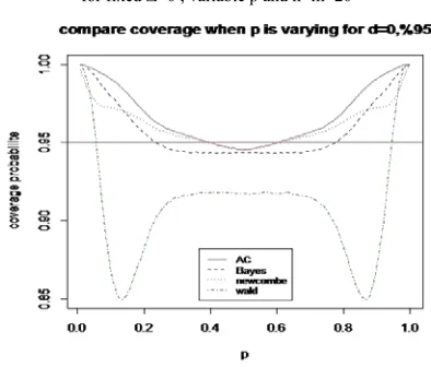
Fig. 4 Compare coverage probability of 95% confidence intervals for fixed ∆=0 , variable p and n=m=20
3.
comparison of confidence interval
of binomial proportion
3.1. Coverage probability of confidence
interval of binomial proportion
consider the coverage probability of CI as follows :
0
( ) ( , ) (1 )
n
k n k k
n
C p I k p p p
k
−
=
= −
∑
Where I(k, p) is equal to one, if CI includes p , otherwise is equal to zero . Figs . 1 and 2 indicate the coverage probability of four CIs for a sample size n=5 and n=50 , respectively . It seems that, except CIw , the other CIs have acceptable
performance in term of coverage probability .
CIA Cand CIBare closer in oscillation to nominal
level, and CIEis upper than nominal level . By
notice to Table 1 , we can see that , CIBhas the less distance of nominal level with respect to other CIs , such as , CIE has the upper nominal level with respect to other CIs .
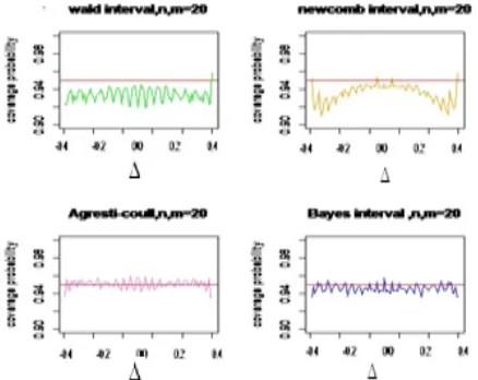
Fig. 5 Compare coverage probability of 95% confidence intervals for variable ∆ , fixed p=0.5 and n=m=20
3.2. Expected length of confidence interval
of binomial proportion
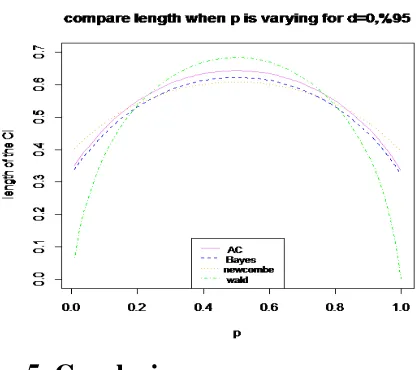
The length of CI is one of the most important performance criteria . In Fig . 3 , four CIs from expected length are in comparison for n=15 , and as it is seen , CIBis shorter than CIEand CIA Cand
this is true even for CIwfor distance of 0.2 until
0.8 . We see that , the CIA Ccan never be shorter
than CIB .
According the Table 2 , we see that , CIwhas the
shortest length in comparison with other intervals in small sample size and it can be argued that , CIBacts as short as CIwand has
much better performance than the other two CIs . But whenever , when the sample size is greater , the difference between CIs becomes less , in term of length criteria . This was expected for us , according to CIs structure.
4. The compare of confidence
interval for difference of two
binomial proportions
4.1. Coverage probability of confidence
interval for difference of two binomial
proportions
With respect to structure of CIs of two binomial proportion , which have four parameters as (m , n , p , ∆) , we compared here , four CIs for different values of their parameters.
Fig . 4 is drown with assumption fixed ∆ and variable p and n=m=20 . Simply it is recognizable that *
new
CI and CI*
Bhave the better
performance than * A g
CI and especially performance than CI*
W .
Fig . 5 is drown for p=0.5 and n=m=20 and for
∆ as a variable , here it is recognizable that ,
* A g
CI has the least oscillation from nominal level , and *
CIW never reach to nominal level and *
new
CI below nominal level is oscillation.
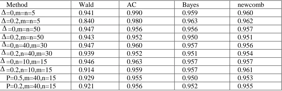
Table 3 indicates the average coverage probability of four CIs in different situation . According on this table , we can remark thatCI*
B
has better performance in average coverage probability than the *
new CI , *
A g
CI and especially
* CIW .
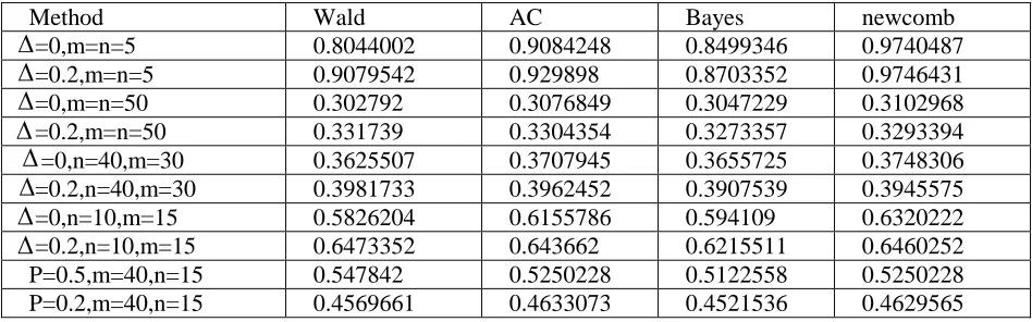
The length of CI is another important attribute in evaluation of a CI . As shown in Fig . 6 and Table 4 , expected length of the CI*
Wis much shorter
than * A g
CI and *
new
CI for smaller sample size . While *
CIBperforms as short as *
CIW in term of
expected length and also , for larger sample their performance is very similar from this viewpoint .
Fig. 6 Compare expected lengths of 95% confidence intervals for ∆=0, n=30 and m=10
5. Conclusion
In this study , we develop by simulation study a CI for binomial proportion and difference of two binomial prop ortions in the hope that , new CI is simple and useful for nearly all sample size . We reviewed the popular CI of binomial proportion and difference of two binomial proportions . By doing similar process we obtained other Bayes CI for binomial proportion and difference of two binomial proportions . Applying of numerical tables and drawing diagrams , we showed that ,
*
CIBhas the good performance in both of the coverage probability and expected length for small sample size . For a larger sample size (>40) except *
CIW , the others CI have acceptable
coverage probability such that , the * A g
CI is
preferred for its simplicity in structure . In this paper we compared CIs of binomial proportion , and indicate the poor performance of CI*
W in
coverage probability . Also for fixed value of p and variable ∆, we recommended the *
A g
CI and
*
CIBwith respect to others . And when the value of ∆ is fixed and parameter p is variable , we proved that , *
new
CI and CI*
Bhave the better
performance than the two other CIs , especially
*
CIW . At last , it is possible that we find out that the CIBand
*
CIBfor all sample sizes in different situation , has better performance from both comparative criteria.
References
[1]A. Agresti, B.A. Coull "Approximation is better than “exact” for interval estimation of binomial proportions", Amer. Statist. 52, 1998, 119–126.
[2] A. Agresti , B. Caffo "Simple effective confidence intervals for proportions and differences of proportions result from adding two successes and two failures." Amer. Statist, 54, 2000, 280–288.
[3] E.B. Wilson, "Probable inference the law of succession and statistical inference, " J. Amer. Statist. Assoc., 22, 1927, 209–212. [4] L. D. Brown, "Confidence interval for two sample binomial distribution", J.Statist Plan. Infer.130, 2004, 359-375.
[5] L. D. Brown, T.T. Caio, A. DasGupta, "Interval estimation for a binomial proportion". Statist. Sci, 16, 2001, 101–133
.
[6] L. D. Brown, T.T. Caio, A. DasGupta, "Confidence intervals for a binomial proportion and asymptotic expansions", Ann. Statist, 30, 2002, 160–201.
[7] R. Newcombe, "Interval estimation for the difference between independent propo- rtionns: comparison of eleven methods", Statist. Med, 17, 1998, 873–890.
First Author: Masoud Ganji is Associate Professor at Department of Statistics, Faculty of Mathematical Science, University of Mohaghegh Ardabili, Ardabil, Iran. He obtained his Ph. D. from the National University of Delhi, India. His research interests are in the areas of Applied Mathematics, Statistical inference. He has published research articles in reputable international journals of Statistics and
sciences. He is referee and editor of mathematical journals in the frame of Applied Mathematics and Statistics. He is currently Director of the journal of Hyperstructures. Second Author: Solmaz Aghlmandi is M.Sc. student of Statistics in the university of Mohaghegh Ardabili, Ardabil, Iran. Her main research interests are Distribution theory, Parameter estimation, Bayes estimation.
Table Titles and Legends
Table 1. Compare coverage probability of 95% confidence intervals for variable n
Method n=5 n=15 n=30 n=40 n=50
Wald 0.651 0.829 0.884 0.901 0.909
AC 0.967 0.963 0.961 0.959 0.957
Bayes 0.950 0.954 0.956 0.955 0.955 Exact 0.990 0.980 0.974 0.971 0.968
Table 2. Compare average expected lengths of 95% confidence intervals for variable
Method n=5 n=15 n=30 n=40 n=50
Wald 0.519 0.365 0.270 0.236 0.212
AC 0.606 0.389 0.280 0.243 0.218
Bayes 0.571 0.379 0.276 0.241 0.216 Exact 0.676 0.418 0.297 0.256 0.228
Table. 3 Compare coverage probability of 95% confidence intervals
Method Wald AC Bayes newcomb
=0,m=n=5 0.941 0.990 0.959 0.960
=0.2,m=n=5 0.840 0.980 0.963 0.962
=0,m=n=50 0.947 0.956 0.956 0.957
=0.2,m=n=50 0.943 0.952 0.950 0.951 =0,n=40,m=30 0.947 0.960 0.957 0.956 =0.2,n=40,m=30 0.939 0.952 0.951 0.954 =0,n=10,m=15 0.946 0.963 0.957 0.957 =0.2,n=10,m=15 0.914 0.959 0.957 0.961 P=0.5,m=40,n=15 0.929 0.955 0.950 0.953 P=0.2,m=40,n=15 0.921 0.956 0.952 0.955
Table. 4 Compare average expected lengths of 95% confidence intervals
Method Wald AC Bayes newcomb
=0,m=n=5 0.8044002 0.9084248 0.8499346 0.9740487 =0.2,m=n=5 0.9079542 0.929898 0.8703352 0.9746431 =0,m=n=50 0.302792 0.3076849 0.3047229 0.3102968 =0.2,m=n=50 0.331739 0.3304354 0.3273357 0.3293394 =0,n=40,m=30 0.3625507 0.3707945 0.3655725 0.3748306 =0.2,n=40,m=30 0.3981733 0.3962452 0.3907539 0.3945575 =0,n=10,m=15 0.5826204 0.6155786 0.594109 0.6320222 =0.2,n=10,m=15 0.6473352 0.643662 0.6215511 0.6460252 P=0.5,m=40,n=15 0.547842 0.5250228 0.5122558 0.5250228 P=0.2,m=40,n=15 0.4569661 0.4633073 0.4521536 0.4629565