Picking the Amateur’s Mind – Predicting Chess Player Strength from
Game Annotations
Christian Scheible
Institute for Natural Language Processing University of Stuttgart, Germany [email protected]
Hinrich Sch¨utze Center for Information and Language Processing University of Munich, Germany
Abstract
Results from psychology show a connection between a speaker’s expertise in a task and the lan-guage he uses to talk about it. In this paper, we present an empirical study on using linguistic evidence to predict the expertise of a speaker in a task: playing chess. Instructional chess litera-ture claims that the mindsets of amateur and expert players differ fundamentally (Silman, 1999); psychological science has empirically arrived at similar results (e.g., Pfau and Murphy (1988)). We conduct experiments on automatically predicting chess player skill based on their natural lan-guage game commentary. We make use of annotated chess games, in which players provide their own interpretation of game in prose. Based on a dataset collected from an online chess forum, we predict player strength through SVM classification and ranking. We show that using textual and chess-specific features achieves both high classification accuracy and significant correlation. Finally, we compare our findings to claims from the chess literature and results from psychology.
1 Introduction
It has been recognized that the language used when describing a certain topic or activity may differ strongly depending on the speaker’s level of expertise. As shown in empirical experiments in psychology (e.g., Solomon (1990), Pfau and Murphy (1988)), a speaker’s linguistic choices are influenced by the way he thinks about the topic. While writer expertise has been addressed previously, we know of no work that uses linguistic indicators to rank experts.
We present a study on predicting chess expertise from written commentary. Chess is a particularly interesting task for predicting expertise: First, using data from competitive online chess, we can compare and rank players within a well-defined ranking system. Second, we can collect textual data for experi-mental evaluation from web resources, eliminating the need for manual annotation. Third, there is a large amount of terminology associated with chess, which we can exploit for n-gram based classification.
Chess is difficult for humans because it requires long-term foresight (strategy) as well as the capacity for internally simulating complicated move sequences (calculationandtactics). For these reasons, the game for a long time remained challenging even for computers. Players have thus developed general principles of chess strategy on which many expert players agree. The dominant expert view is that the understanding of fundamental strategical notions, supplemented by the ability of calculation, is the most important skill of a chess player. A good player develops a long-termplanfor the course of the game. This view is the foundation of many introductory works to chess (e.g., Capablanca (1921), one of the earliest works).
Silman (1999) presents games he played with chess students, analyzing their commentary about the progress of the game. He claims that players who fail to adhere to the aforementioned basic princi-ples tend to perform worse and argues that the students’ thought processes reflect their playing strength directly. Lack of strategical understanding marks the difference between amateur and expert players. Experts are mostly concerned withpositionalaspects, i.e., the optimal placement of pieces that offers a
This work is licenced under a Creative Commons Attribution 4.0 International License. Page numbers and proceedings footer are added by the organizers. License details:http://creativecommons.org/licenses/by/4.0/
8
rm0ZkZ0s
7
opo0lpa0
6
0Z0ZpZpo
5
Z0Z0O0Z0
4
0Z0Z0ZbZ
3
Z0MBZNZ0
2
POPZ0OPO
1
S0ZQZRJ0
[image:2.595.210.379.61.236.2]a b c d e f g h
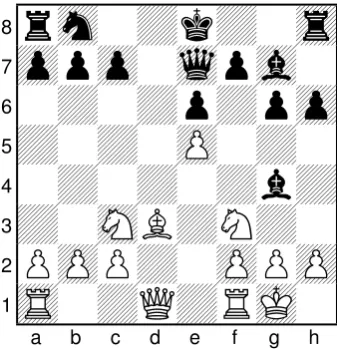
Figure 1: Example chess position, white to play
long-lasting advantage. Amateurs often havetacticalaspects in mind, i.e., short-term attacking oppor-tunities and exploits that potentially lead to loss of material for their opponents. A correlation between chess strength and verbalization skills has been shown empirically by Pfau and Murphy (1988), who used experts to assess the quality of the subjects’ writing.
In this paper, we investigate the differences between the mindset of amateurs and experts expressed in written game commentary, also referred to asannotated games. When studying chess, it is best practice to review one’s own games to further one’s understanding of the game (Heisman, 1995). Students are encouraged toannotatethe games, i.e., writing down their thought process at each move. We address the problem of predicting the player’s strength from the text of these annotations. Specifically, we want to predict the rank of the player at the point when a given game was played. In competitive play, the rank is determined through a numerical rating system – such as the Elo rating system (Elo, 1978) used in this paper – that measures the players’ relative strength using pairwise win expectations.
This paper makes the following contributions. First, we introduce a novel training dataset of games annotated by the players themselves – collected from online chess forum. We then formulate the task of playing strength prediction. For each annotated game, each game viewed as a document, we predict the rating class or overall rank of the player. We show that (i) an SVM model with n-gram features succeeds at partitioning the players into two rating classes (above and below the mean rating); and (ii) that ranking SVMs achieve significant correlation between the true and predicted ranking of the players. In addition, we introduce novel chess-specific features that significantly improve the results. Finally, we compare the predictions made by our model to claims from instructional chess literature and results from psychology research.
We next give an overview of basic chess concepts (Section 2). Then, we introduce the dataset (Sec-tion 3) and task (Sec(Sec-tion 4). We present our experimental results in Sec(Sec-tion 5. Sec(Sec-tion 6 contains an overview of related work.
2 Basic Chess Concepts
2.1 Chess Terminology
We assume that the reader has basic familiarity with chess, its rules, and the value of individual pieces. For clarity, we review some basic concepts of chess terminology, particularly elementary concepts related to tactics and strategy in an example position (Figure 1).1
From a positional point of view, white is ahead in development: all hisminor pieces (bishops and knights) have moved from their starting point while black’s knight remains on b8. White has alsocastled
(a move where the rook and king move simultaneously to get the king to a safer spot on either side of the board) while black has not. White has aspaceadvantage as he occupies the e5-square (which is in black’s
1.e4 e5 2.Nf3 Nc6 3.Bc4 Nh6 4.Nc3 Bd6 Trying to follow basic opening principals, control center, develop. etc5.d3 Na5 6.Bb5Moved bishop not wanting to trade, but realized after the move that my bishop would be harassed by the pawn on c7 6...c6 7.Ba4Moved bishop to safety, losing tempo7...Qf6 8.Bg5 Qg6 9.O-O b5Realized my bishop was done, might as well get 2 pawns 10.Nxb5 cxb5 11.Bxb5 Ng4 12.Nxe5Flat out blunder, gave up a knight, at least I had a knight I could capture back 12...Bxe5 13.Qxg4 Bxb2 14.Rab1 Bd4 15.Rfe1Moved rook to E file hoping to eventually attack the king. 15...h6 16.c3 Poor attempt to move the bishop, I realized it after I made the move 16...Bxc3 17.Rec1 Be5 18.d4Another crappy attempt to move that bishop18...Bxd4 19.Rd1 O-O 20.Rxd4 d6 21.Qd1I don’t remember why I made this move. 21...Qxg5 22.Rxd6 Bh3 23.Bf1Protecting g2 23...Nc4 24.Rd5 Qg6 25.Rc1 Qxe4 26.f3 Qe3+ 27.Kh1 Nb2 28.Qc2 Rac8 29.Qe2 Qxc1 30.gxh3 Nc4 31.Qe4 Qxf1#
Figure 2: Example of an annotated game from the dataset (by user aevans410, rated 974)
half of the board) with a pawn. This pawn is potentiallyweakas it cannot easily be defended by another pawn. Black has both of his bishops (the bishop pair) which is considered advantageous as bishops are often superior to knights in open positions. Black’s light-square bishop isbadas it is obstructed by black’s own pawns (although it is outside thepawn chainand thus flexible). Strategically, black might want to improve the position of the light-square bishop, make use of his superior dark-square bishop, and try to exploit the weak e5 pawn. Conversely, white should try create posts for his knights in black’s territory. Tactically, white has an opportunity to move his knight to b5 (written Nb5 in algebraic chess notation), from where it would attack the pawn on c7. If the knight could reach c7 (currently defended by black’s queen), it wouldfork(double attack) black’s king and rook, which could lead to the trade of the knight for the rook on the next move (which is referred to as winning theexchange). White’s knight on f3 ispinned, i.e., the queen would be lost if the knight moved. Black can win a pawn byremoving the defenderof e5, the knight on f3, by capturing it with the bishop.
This brief analysis of the position shows the complex theory and terminology that has developed around chess. The paragraph also shows an example of game annotation (although not every move in the game will be covered as elaborately in practice in amateur analyses).
2.2 Elo Rating System
Our goal in this paper is to predict the ranking of chess players based on their game annotations. We will give a brief overview of the Elo system (Elo, 1978) that is commonly used to rank players. Each player is assigned a score that is changed after each game depending on the expected and actual outcome. On
chess.com, a new player starts with an initial rating of 1200 (an arbitrary number chosen for historical reasons, which has since become a wide-spread convention in chess). Assuming the current ratingsRa andRbof two playersaandb, the expected outcome of the game is defined as
Ea= 1
1 + 10−Ra400−Rb .
Ea is then used to conduct a (weighted) update of Ra andRb given the actual outcome of the game. Thus, Elo ratings make pairwise adjustments to the scores. The differences between the ratings of two players predict the probability of one winning against the other. However, the absolute ratings do not carry any meaning by themselves.
3 Annotated Chess Game Data
For supervised training, we require a collection of chess games annotated by players of various strengths. An annotated chess game is a sequence of chess moves with natural language text commentary associated to specific moves. While many chess game collections are available, some of them containing millions of games, the majority are unannotated. The small fraction of annotated games mostly features commentary by masters rather than amateurs, which is not interesting for a contrastive study.
Parameter Value
# games 182
[image:4.595.182.401.61.387.2]# different players 130 mean # moves by game 42 mean # annotated moves by game 16 mean # words by game 114
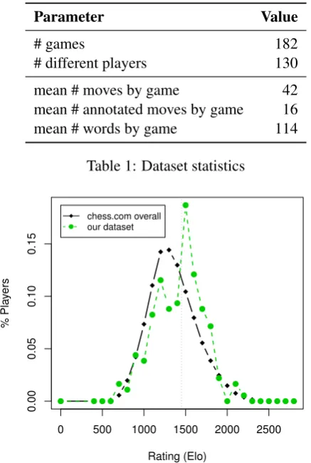
Table 1: Dataset statistics
0 500 1000 1500 2000 2500
0.00
0.05
0.10
0.15
Rating (Elo)
% Pla
yers
● ● ● ● ●
● ●
● ●
●
●● ●
●
●
●
●
● ●
●
● ● ● ● ● ● ● chess.com overallour dataset
Figure 3: Rating distribution on chess.com and our dataset.4 Each point shows the percentage of
players in a bin of width 50 around the value. Dotted line: Median on our dataset used for binning.
Many games are posted without annotations, instead soliciting annotation from the community. Others are missing the rating of the player at the time the game was played – the user profile shows only the current rating for the player which may differ strongly from their historical one.
We first downloaded all available games from the forum archive. The games are stored in portable game notation (PGN, Edwards (1994)). Next, we manually removed games where the annotation had been conducted automatically by a chess program. We also removed games that had annotations at fewer than three moves. The final dataset consists of 182 games with annotations in English and known player rating.2 We reproduce an example game from the data in Figure 2. This game is typical as the first couple of moves are not commented (as opening moves are typically well-known). Then, the annotator comments on select moves that he believes are key to the progress of the game. Table 1 shows some statistics about the dataset.
The distribution of the ratings in our dataset is shown in Figure 3 in comparison to the overall standard chess rating distribution onchess.com.3 Elo ratings assume a normal distribution of players. We see that overall, the distributions are quite similar, although we have a higher peak and our sample mean is shifted towards higher ratings (1347 overall vs 1462 on our dataset). It is more common for mid-level players to request annotation advice than it is for low-rated players (who might not know about this practice) or high-rated players (who do not look for support by the lower-rated community).
The dataset is still somewhat noisy as players may obtain different ratings depending on the type of venue (over-the-board tournament vs online chess) or the amount of time the players had available (time control). Differences in these parameters lead to different rating distributions.4 For this reason, the total ordering given through the ratings may be difficult to predict. Thus, we will conduct experiments both
2Available athttp://www.ims.uni-stuttgart.de/data/chess 3Data fromhttp://www.chess.com/echess/players
on ranking and on classification where the rating range is binned into two rating classes.
4 Predicting Chess Strength from Annotations
4.1 Classification and Ranking
The task addressed in this paper is prediction on the game level, i.e., predicting the strength of the player of each game at the time when the game was played. We view a game as a document – the concatenation of the annotations at each move – and extract feature vectors as described in Section 4.2. We pursue two different machine learning approaches based on support vector machines (SVMs) to predicting chess strength: classification and ranking.
The simplest way to approach the problem is classification. For this purpose, we divide the range of observed rating into two evenly spaced rating classes at the median of the overall rating range (henceforth
amateurandexpert). The classification view has obvious disadvantages. At the boundaries of the bins, the distinction between them becomes difficult.
To predict a total ordering of all players, we use a ranking SVM (Herbrich et al., 1999). This model casts ranking as learning a binary classification function that decides whetherrank(x1)>rank(x2)over
all possible pairs of example feature vectorsx1andx2 with differingrank.
Note that since Elo ratings are continuous real numbers, it would be conceivable to fit a regression model. However, Elo is designed as a pairwise ranking measure. While a relative difference in Elo represents the probability of one player beating the other, the absolute Elo rating is not directly inter-pretable.5
4.2 Features
We extract unigrams (UG) and bigrams (BG) from the texts. In addition, we propose the following two chess-specific feature sets derived from the text:6
Notation (NOT). We introduce two indicators for whether the annotations contain certain types of
formal chess notation. The featureSQUAREis added if the annotation contains a reference to a specific square on the chess board (e.g.,d4). If the annotation contains a move in algebraic notation (e.g.,Nxb4+, meaning that a knight moved to b4, captured a piece there and put the enemy king in check), the feature MOVEis added.
Similarity to master annotations (MS). This feature is intended to compensate for the lack of training
data. We used a master-annotated database consisting of 500 games annotated by chess masters which is available online.7 As we do not know the exact rating of the annotators, and to avoid strong class imbalances, we cannot make use of the games directly through supervision. Instead, we calculate the cosine similarity between the centroid8of the n-gram feature vectors of the master games and each game in thechess.comdataset. The cosine similarity between each game and the master centroid is added as a numerical feature.
Additionally, the master similarity scores can be used on their own to rank the games. This can be viewed distant supervision as strength is learned from an external database. We will evaluate this ranking in comparison with our trained models.
5 Experiments
This section, contains experimental results on classifying and ranking chess players. We first present quantitative evaluation of the classification and ranking models and discuss the effect of chess-specific
5Preliminary experiments with SVM regression showed little improvements over a baseline of assigning the mean rating to
all games. This suggests that the distribution of rankings is difficult to model – possibly due to the low number of annotated games on which the model can be trained.
6We also tried using the length of the annotation as well as the number of annotated moves as a feature, which did not
contribute any improvements.
7http://www.angelfire.com/games3/smartbridge/famous_games.zip
8We also tried ak-NN approach where we computed the mean similarity of a game from our dataset to itsk nearest
Model Features F1(↓) F1(↑) F1(∅)
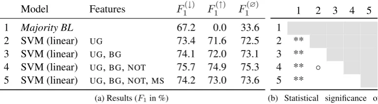
1 Majority BL 67.2 0.0 33.6
2 SVM (linear) UG 73.4 71.6 72.5 3 SVM (linear) UG,BG 74.1 72.0 73.1 4 SVM (linear) UG,BG,NOT 75.7 74.9 75.3 5 SVM (linear) UG,BG,NOT,MS 74.2 73.0 73.6
(a) Results (F1in %)
1 2 3 4 5
1 2 ** 3 ** 4 ** ◦
5 **
[image:6.595.92.504.66.274.2](b) Statistical significance of differences inF1. **:p <0.01, *:p <0.05,◦:p <0.1
Table 2: Classification results
Class Features
Amateur (↓) bishop, d4, opening, instead, trying, should, did, where, do, even, rook, get, good, he, coming, point i, exchange, thought, did not, his, clock, too, or, on clock, knight for
Expert (↑) this, game, can, will, winning,NOT:move, time, draw, because, white, back, black, mate, that, but, moves, can’t, very, on, won, really, so, i know, now, only
Table 3: Top 25 features with most negative (amateur) and positive (expert) weights (mean over all folds) in the best setup (UG,BG,NOT)
features. Second, we qualitatively compare the predictions of our models with findings and claims from the literature about the connection between a player’s mindset and strength.
5.1 Experimental Setup
To generate feature vectors, we first concatenate all the annotations for a game, tokenize and lowercase the texts, and remove punctuation as well as a small number of stopwords. We exclude rare words to avoid overfitting: We remove all n-grams that occur fewer than 5 times, and add the chess-specific features proposed above. Finally, weL2-normalize each vector.
We use linear SVMs from LIBLINEAR and SVMs with RBF kernel from LIBSVM (Chang and Lin, 2011). We run all experiments in a 10-fold cross-validation setup.
We measure macro-averagedF1for our classification results. We evaluate the ranking model using two
measures: pairwise ranking accuracy (Accr), i.e., the accuracy over the binary ranking decision for each player pair; and Spearman’s rank correlation coefficientρfor the overall ranking. To test whether differ-ences between results are statistical significant, we apply approximate randomization (Noreen, 1989) for
F1, and the test by Steiger (1980) for correlations, which is applicable toρ.
5.2 Classification
We first investigate the classification case, i.e., whether we can distinguish players below and above the rating mean. Table 2 shows the results for this experiment. We showF1 scores for the lower and higher
half of the players (F1(↓)andF1(↑), respectively), and the macro average of these two scores (F1(∅)). We first note that all SVM classifiers (lines 2–5) score significantly higher than the majority baseline (line 1). When adding bigrams (line 3) and chess-specific notation features (line 4),F1increases. However, these
improvements are not statistically significant. The master similarity feature (line 5) leads to a drop in
F1from the previous line. The relatively low rank correlation between the master similarity scores and
the two classes (ρ= 0.334) leads to this effect. The low correlation itself may occur because the master games were annotated by a third party (instead of the players), leading to strong differences in style.
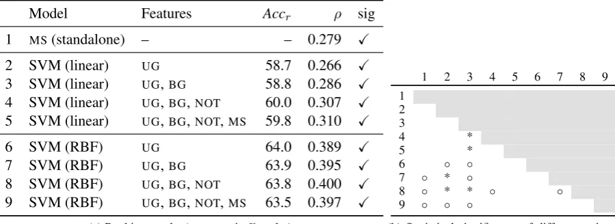
[image:6.595.106.494.68.175.2]Model Features Accr ρ sig
1 MS(standalone) – – 0.279 �
2 SVM (linear) UG 58.7 0.266 �
3 SVM (linear) UG,BG 58.8 0.286 � 4 SVM (linear) UG,BG,NOT 60.0 0.307 � 5 SVM (linear) UG,BG,NOT,MS 59.8 0.310 �
6 SVM (RBF) UG 64.0 0.389 �
7 SVM (RBF) UG,BG 63.9 0.395 �
8 SVM (RBF) UG,BG,NOT 63.8 0.400 � 9 SVM (RBF) UG,BG,NOT,MS 63.5 0.397 �
(a) Ranking results (accuracy in % andρ)
1 2 3 4 5 6 7 8 9
1 2 3
4 *
5 *
6 ◦ ◦
7 ◦ * ◦
8 ◦ * * ◦ ◦
9 ◦ ◦ ◦
[image:7.595.77.527.63.227.2](b) Statistical significance of differences in ρ. **:p <0.01, *:p <0.05,◦:p <0.1
Table 4: Ranking results for standalone master similarity and SVM (linear and RBF kernel). Check in sig column denote significance of correlation with true ranking (p <0.05). Numbers in sigdiff column denote a significant improvement (p <0.05) inρover the respective line.
find that there are noticeable differences in the writing styles of amateurs and experts. According to the model, one of the most prominent distinctions is that amateurs tend to refer to the opponent ashe, whereas experts usewhiteandblackmore frequently. However, it is of course not universally true, which leads to the misclassification of some experts as amateurs. Another difference in style is that amateur players tend to write about the game in the past tense. This is a manifestation of an important distinction: Amateurs often state the obvious developments of the game (e.g., Flat out blunder, gave up a knight
in Figure 2) or speculate about options (e.g., hoping to eventually attack), while experts provide more thorough positional analysis at key points.
5.3 Ranking
We now turn to ranking experiments (Table 4). We first evaluate the ranking produced by ordering the games by their similarity to the master centroid (line 1). We find that the resulting rank correlation is low but significant.
The results for the linear SVM ranker are shown in lines 2–5. Total ranking is considerably more diffi-cult than binary classification of rating classes. Using a linear SVM, we again achieve low but significant correlations. The linear classifiers (lines 2–5) do not significantly outperform the standalone master sim-ilarity (MS) baseline (line 1). Chess-specific features (lines 4 and 5) boost the results, outperforming the bigram models (line 3) significantly. The improvement from adding theMScentroid score feature is not significant.
We again perform error analysis by examining the feature weights (Table 5). We find an overall picture similar to the classification setup (cf. Table 3). The notation feature serves as a good indicator for the upper rating range (cf. Table 3) as experienced players find it easier to express themselves through notation. We observed that lower players tend to express moves in words (e.g., “move my knight to d5”) rather than through notation (Nd5), which could serve as an explanation for why pieces (bishop,knight,
rook) appear among the top features for amateur players.
However, some features change signs between the two experiments (e.g., king,square). This effect may indicate that the binary ranking problem is not linearly separable, which is plausible; mid-rated players may use terms that neither low-rated nor high-rated players use. Examining correlations at dif-ferent ranking ranges confirms this suggestion. In top and bottom thirds of the rating scale, the true and predicted ranks are not correlated significantly. This means that the ranking SVM only succeeds at rank-ing players in middle third of the ratrank-ing scale. To introduce non-linearity, we conduct further experiments with an SVM with a radial basis function (RBF) kernel.
Class Features
Weaker instead, king, thinking, one my, fight, d4, even, should, should i, bishop, decided, did, i didn’t, opening, feel, put, defense, knight on, black king, been, with my, where, get, cover, pin
[image:8.595.159.518.172.337.2]Stronger NOT:move, moves, game, time, won, i know, already, will, stop, way, winning, line, can’t, can, black has, this, MS, king side, computer, threaten, first, back, any way, my knight, win pawn, d
Table 5: Top 25 features with most negative (lower rating) and positive (higher rating) weights, mean over all folds (rank(x1)>rank(x2)or vice versa) in the best ranking setup (linear SVM,UG,BG,NOT)
Feature Coefficient capture -0.29 take -0.21 bishop -1.06 knight -0.19 rook -0.54 king 0.19 queen 0.08 pawn 0.44 pin -0.26 fork -0.27 Feature Coefficient threat 0.13 danger 0.25 stop 0.50 weakness 0.34 light 0.21 dark 0.37 variation 0.41 winning 0.87 losing 0.08 like -0.16 hate -0.05 good -0.27 bad 0.52 Feature Coefficient white 0.74 black 0.71 he -0.51 fight -0.17 know 0.41 will 0.88 thinking -0.44 believe -0.02 maybe -0.19 hoping -0.30 Feature Coefficient time 0.81 clock -0.47
time pressure -0.12
blunder -0.31 tempo -0.36 checkmate -0.24 mate 0.69 opening -0.63 castle -0.33 fall -0.22 eat -0.28
Table 6: Selected SVM weights in the best 2-class setup, mean over all folds
the unigram and bigram linear models; all except for the unigram model (lines 7–9) also yield weakly significant improvements over theMSbaseline. Adding the notation features (line 8 improves the results and leads to improvements with stronger significance. The RBF kernel makes feature weight analysis impossible, so we cannot perform further error analysis.
5.4 Comparing the Learned Models and Strength Indicators from the Chess Literature
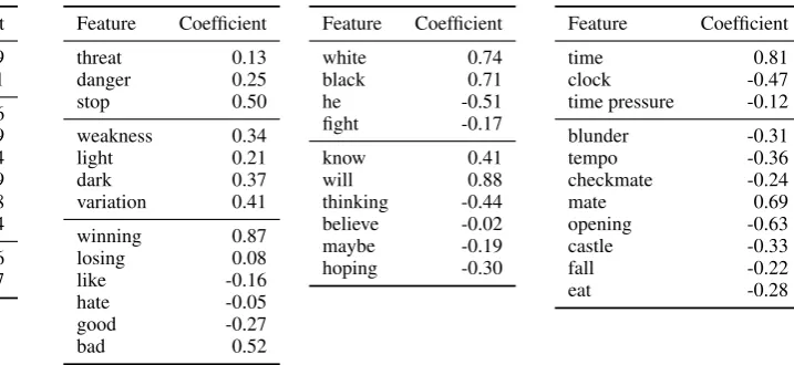
There are many conjectures from instructional chess literature and results from psychological research about various aspects of player behavior. In this section, we compare these to the predictions made by our supervised expertise model. In Table 6, we list selected weights from the best classification model (line 3 in Table 2). We opt for analzying the classifier rather than the ranker as we find the former more directly interpretable.
Long-Term vs Short-Term Planning. The SVM model reflect the short-term nature of the amateurs’ thoughts in several ways: (i) Amateurs focus on specific moves rather than long-term plans, and thus, terms like capture andtake are deemed predictive for lower ratings. (ii) Amateurs often think piece-specific (Silman, 1999), particularly about moves with minor pieces (bishoporknight), and these terms receive high negative weights, pointing to lower ratings. Related to this, Reynolds (1982) observed that amateurs often focus on the current location of a piece, whereas experts mostly consider possible future locations. The SVM model learns this by weighting bigrams of the form* on, where* is a piece, as indicators for low ratings. (iii) Many terms related to elementary tactics (e.g.,pin,fork) indicate lower-rated players, whereas terms relating to tactical foresight (e.g.,threat,danger,stop) as well as positional terms (e.g.,weakness,lightanddarksquares,variation) indicate higher-rated players.
Emotions. A popular and wide-spread claim is that weaker chess players often lose because they are too emotionally invested in the game and thus get carried away (e.g., Cleveland (1907), Silman (1999)). We experimented with a sentiment feature, counting polar terms in the annotations using a polarity lexicon (Wilson et al., 2005). However, this feature did not improve our results.
players while it is open for weaker ones. Expert players tend to assess positions aswinningorlosing
for a side, whereas weaker players tend to use terms such aslikeandhate. Both terms are identified as indicators of the respective strength class in our models. Other subjective assessments (e.g.,good and
bad) are divided among the classes. Emotional tendencies of amateurs can also be observed through objective indicators. As discussed above, stronger players talk about the game with a more distanced view, often referring to their opponent by their color (whiteorblack) rather than using the pronounhe. Lower-rated players appear to use terms indicating competitions more frequently, such asfight.
Confidence. Silman (1999) argues that weaker players lack confidence, which leads to them losing track of their own plans and to eventually follow their opponent’s will (often calledlosing the initiative). This process is indeed captured by our trained models. Terms of high confidence (such asknow,will) are weighted towards the stronger class, whereas terms with higher uncertainty (such asthinking,believe,
maybe, hoping) indicate the weaker class. This observation is in line with findings on self-assigned confidence judgments of chess players (Reynolds, 1992). The sets of terms expressing certainty and uncertainty, respectively, are small in our dataset, so weights for most terms can be learned directly on the n-grams.
Time Management. It has been suggested that deficiencies in time management are responsible for many losses at the amateur level, particularly in fast games (e.g., blitz chess, where each player has 5 minutes to complete the game), for example due to poor pattern recognition skills of beginners (Calder-wood et al., 1988). In the trained models, we see that the termtimeitself is actually considered a good indicator for stronger players.Timeis often used to signify number of moves. So, when used on its own,
timeis referring to efficient play, which is indicative of strong players. Conversely, the termsclockand
time pressureare deemed good features to identify weaker players.
Chess Terminology. As shown in Section 2.1 and throughout this paper, there is a vast amount of chess terminology. We observe that frequent usage of such terms (e.g.,blunder– a grave mistake,tempo, check-mate– experts usemate,opening,castle) actually indicate a weaker player. This seems counterintuitive at first, as we may expect lower-rated players to be less familiar with such terms. However, it appears that they are frequently overused by weaker players. This also holds for metaphorical terms, such asfall
oreatinstead ofcapture.
6 Related Work
The treatment of writer expertise in extralinguistic tasks in NLP has mostly focused on two problems: (i) retrieval of experts for specific areas – i.e., predicting the area of expertise of a writer (e.g., Tu et al. (2010; Kivim¨aki et al. (2013)); and (ii) using expert status in different downstream applications such as sentiment analysis (e.g., Liu et al. (2008)) or dialog systems (e.g., Komatani et al. (2003)). Conversely, our work is concerned with predicting a ranking by expertise within a single task.
Several publications have dealt with natural language processing related to games. Chen and Mooney (2008) investigate grounded language learning where commentary describing the specific course of a game is automatically generated. Commentator expertise is not taken into account in this study. Branavan et al. (2012) introduced a model for using game manuals to increase the strength of a computer playing the strategy video gameCivilization II. Cadilhac et al. (2013) investigated the prediction of player actions in the strategy board gameThe Settlers of Catan. Our approach differs conceptually from theirs as their main focus lies on modeling concreteactionsin the game (either predicting or learning them); our goal is to predictplayer strength, i.e., to learn to compare players among each other. Rather than explicitly modeling the game, commentary analysis aims to provide insight into specific thought processes.
7 Conclusion
In this paper, we presented experiments on predicting the expertise of speakers in a task using linguistic evidence. We introduced a classification and a ranking task for automatically ranking chess players by playing strength using their natural language commentary. SVM models succeed at predicting either a rating class or an overall ranking. In the ranking case, we could significantly boost the results by using chess-specific features extracted from the text. Finally, we compared the predictions of the SVM with popular claims from instructional chess literature as well as results from psychology research. We found that many of the traditional findings are reflected in the features learned by our models.
Acknowledgements
We thank Daniel Quernheim for providing his chess expertise, Kyle Richardson and Jason Utt for helpful suggestions, and the anonymous reviewers for their comments.
References
SRK Branavan, David Silver, and Regina Barzilay. 2012. Learning to win by reading manuals in a monte-carlo framework. Journal of Artificial Intelligence Research, 43(1):661–704.
Anais Cadilhac, Nicholas Asher, Farah Benamara, and Alex Lascarides. 2013. Grounding strategic conversation: Using negotiation dialogues to predict trades in a win-lose game. InProceedings of the Conference on Empirical Methods in Natural Language Processing (EMNLP), pages 357–368.
Roberta Calderwood, Gary A Klein, and Beth W Crandall. 1988. Time pressure, skill, and move quality in chess.
The American Journal of Psychology, 101(4):481–493. Jos´e R Capablanca. 1921.Chess Fundamentals. Harcourt.
Chih-Chung Chang and Chih-Jen Lin. 2011. LIBSVM: A library for support vector machines. ACM Transactions on Intelligent Systems and Technology (ACM TIST), 2(3):1–27.
David L Chen and Raymond J Mooney. 2008. Learning to sportscast: a test of grounded language acquisition. In
Proceedings of the 25th International Conference on Machine learning (ICML), pages 128–135.
Alfred A Cleveland. 1907. The psychology of chess and of learning to play it. The American Journal of Psychol-ogy, 18(3):269–308.
Steven J Edwards. 1994. Portable game notation specification and implementation guide. Arpad E Elo. 1978. The Rating of Chessplayers, Past and Present. Batsford.
Dan Heisman. 1995. The Improving Annotator – From Beginner to Master. Chess Enterprises.
Ralf Herbrich, Thore Graepel, and Klaus Obermayer. 1999. Large margin rank boundaries for ordinal regression.
Advances in Neural Information Processing Systems (NIPS), pages 115–132.
Ilkka Kivim¨aki, Alexander Panchenko, Adrien Dessy, Dries Verdegem, Pascal Francq, Hugues Bersini, and Marco Saerens. 2013. A graph-based approach to skill extraction from text. InProceedings of TextGraphs-8, pages 79–87.
Kazunori Komatani, Shinichi Ueno, Tatsuya Kawahara, and Hiroshi G. Okuno. 2003. Flexible guidance genera-tion using user model in spoken dialogue systems. InProceedings of the 41st Annual Meeting of the Association for Computational Linguistics (ACL), pages 256–263.
Yang Liu, Xiangji Huang, Aijun An, and Xiaohui Yu. 2008. Modeling and predicting the helpfulness of online reviews. In Proceedings of the 2008 Eighth IEEE International Conference on Data Mining (ICDM), pages 443–452.
Eric W Noreen. 1989. Computer Intensive Methods for Hypothesis Testing: An Introduction. Wiley.
Robert I Reynolds. 1982. Search heuristics of chess players of different calibers. The American journal of psychology, 95(3):383–392.
Robert I Reynolds. 1992. Recognition of expertise in chess players. The American journal of psychology, 105(3):409–415.
Jeremy Silman. 1999.The Amateur’s Mind: Turning Chess Misconceptions into Chess Mastery. Siles Press. Gregg E A Solomon. 1990. Psychology of novice and expert wine talk. The American Journal of Psychology,
103(4):495–517.
James H Steiger. 1980. Tests for comparing elements of a correlation matrix. Psychological Bulletin, 87(2):245. Yuancheng Tu, Nikhil Johri, Dan Roth, and Julia Hockenmaier. 2010. Citation author topic model in expert search.
InProceedings of the 2010 Conference on Computational Linguistics (Coling): Posters, pages 1265–1273. Theresa Wilson, Janyce Wiebe, and Paul Hoffmann. 2005. Recognizing contextual polarity in phrase-level