S
URFACE
M
ASS
L
OADING TO
C
ONSTRAIN THE
E
LASTIC
S
TRUCTURE OF THE
C
RUST AND
M
ANTLE
Thesis by
Hilary Rose Martens
In Partial Fulfillment of the Requirements for the Degree of
Doctor of Philosophy
California Institute of Technology Pasadena, California
2016
c
2016
Hilary Rose Martens
ORCID: 0000-0003-2860-9013
Acknowledgments
This thesis would not have been possible without support, inspiration, and guidance from many colleagues, mentors, friends, and family. Since I have limited space with which to express my gratitude, suffice to say that the immeasurable contributions of countless individuals have not gone unnoticed and are deeply appreciated.
First of all, I thank my primary research adviser, Professor Mark Simons, for introducing me to interesting topics in geodesy and surface mass loading. Despite the inevitable challenges of research, Mark provided me with consistent motivation and encouragement throughout the five years of this project. He believed in the value of our work, even when I failed to see the value in it myself at times. I am grateful to have had the opportunity to learn from Mark’s tremendous expertise and scientific creativity, particularly on the subject of geophysical inverse problems.
I am also deeply indebted to my honorary adviser, mentor, and friend, Professor Luis Rivera of the University of Strasbourg, for his extraordinary kindness and generosity. Through in-numerable hours of patient instruction, Luis shared with me his expert knowledge of Earth deformation and numerical modeling, which shaped a significant portion of my thesis re-search and led to the development of our software suite,LoadDef. Luis has an extraor-dinary ability to distill difficult concepts into a fundamental form and to convey the infor-mation clearly and coherently. I am grateful for his support and continually inspired by his positivity, modesty, and passion for science.
In addition, I appreciate the ongoing support of my thesis advisory committee: Jennifer Jackson, Michael Gurnis, and Victor Tsai. Susan Owen of the Jet Propulsion Laboratory graciously mentored me on application-specific methods of GPS data processing. Duncan Agnew, Richard Ray, Takeo Ito, Jean-Paul Boy, and Shailen Desai, among others, con-tributed substantially to my understanding of ocean tidal loading and related phenomena.
who laid the foundation for my doctoral work: Bob White (Cambridge University), Geraint Jones (University College London), Andrew Coates (Mullard Space Science Laboratory), and Daniel Reisenfeld (University of Montana). Moreover, I thank the Marshall Aid Com-memoration Commission for providing academic, personal, and financial support during my studies in the United Kingdom as well as the staff and donors of the Davidson Honors College for facilitating my academic and research pursuits as an undergraduate student at the University of Montana.
I am grateful to my friends and colleagues who helped me to find balance in life over the years, including through music, outdoor adventures, coffee chats, and traveling. I also thank the Caltech Residence Life staff, students of Ruddock House, and the residents of Marks and Braun for welcoming me into their communities. Serving as a Resident Associate has been a most meaningful experience for me during the past four years.
In its early stages, this research was supported by the National Science Foundation under grant number DGE-1144469. Subsequent support from the NASA Earth and Space Science Fellowship commenced in September 2014 under grant number NNX14AO04H and from the National Science Foundation Geophysics Program under grant number EAR-1417245.
Abstract
Published Content and Contributions
* Figure 1.1 reproduced and modified with permission from Agnew (2015).
* Figure 8.6 reproduced and modified with permission from Williams & Penna (2011).
* The work described in Chapter 6 has been accepted for publication byJournal of Geo-physical Research. The current reference is: Martens, H.R., L. Rivera, M. Simons, and
T. Ito, 2016. The sensitivity of surface mass loading displacement response to perturba-tions in the elastic structure of the crust and mantle, J. Geophys. Res. Solid Earth, 121, doi:10.1002/2015JB012456.|H.R.M. co-wrote and implemented the software used to com-pute the load Love numbers, load Green’s functions, and predicted load-induced surface displacements; generated the figures; analyzed the results; and wrote the manuscript.
* The work described in Chapter 7 has been published in Geophysical Journal Interna-tional. The reference is: Martens, H.R., M. Simons, S. Owen, and L. Rivera, 2016.
Contents
Abstract v
Published Content and Contributions vi
1 Tidal Theory 1
1.1 Introduction and Motivation . . . 1
1.2 Tide-Generating Forces . . . 3
1.3 Tidal Potential . . . 7
1.4 Equilibrium Tide Formulation . . . 12
1.4.1 Direct Mathematical Approach . . . 12
1.4.2 Harmonic Decomposition Approach . . . 18
1.5 Tidal Potential Catalogues . . . 23
1.6 Physical Interpretation of Tidal Harmonics . . . 26
1.7 Tidal Dynamics . . . 31
1.8 Suggestions for Further Reading . . . 33
2 Harmonic Analysis 34 2.1 Introduction . . . 34
2.2 Harmonic Modulations and Corrections . . . 36
2.2.1 Example: L2 Harmonic . . . 44
2.3 Shallow-Water Harmonics . . . 48
2.4 Constituent Selection . . . 53
2.5 Inversion . . . 55
2.6 Error Analysis . . . 59
2.7 Particle Motion Ellipses . . . 60
2.8 Suggestions for Further Reading . . . 63
3 GNSS-Inferred Measurements of Ocean Tidal Loading Response 64 3.1 Introduction . . . 64
3.2 Basic GPS Theory . . . 65
3.3 Data Acquisition and Formatting . . . 67
3.4 GPS Data Processing Strategies . . . 67
3.4.2 Recovery of the OTL-Response Signal . . . 69
3.4.3 Removal of the Solid Earth Body Tides . . . 71
3.5 Post-Processing Techniques . . . 71
3.5.1 Cleaning the Time Series . . . 71
3.5.2 Spectral Analysis . . . 72
3.5.3 Removal of Non-OTL Mass Loading Signals . . . 72
4 Modeling Earth Deformation Induced by Surface Mass Loading 74 4.1 Introduction . . . 74
4.2 Love Number Computation . . . 75
4.2.1 Introduction . . . 75
4.2.2 Equilibrium Equations for Material Deformation . . . 77
4.2.3 Conversion to Spherical Coordinates . . . 81
4.2.4 Linear Elastic Constitutive Relation . . . 87
4.2.5 Solutions to the Equations of Motion . . . 90
4.2.6 Reduction of the Equations of Motion to First Order . . . 96
4.2.7 Non-dimensionalization . . . 99
4.2.8 Starting Solutions: Power Series Expansion . . . 99
4.2.9 Starting Solutions: Homogeneous Sphere . . . 105
4.2.10 Starting Solutions: Approximation . . . 107
4.2.11 Runge-Kutta Integration . . . 107
4.2.12 Fluid Layers . . . 108
4.2.13 Boundary Conditions at Solid-Fluid Interfaces . . . 110
4.2.14 Surface Boundary Conditions . . . 111
4.2.15 Load Love Numbers . . . 117
4.2.16 Potential Love Numbers . . . 118
4.2.17 Shear Love Numbers . . . 119
4.2.18 Stress Love Numbers and Degree-1 Modes . . . 119
4.2.19 Numerical Considerations . . . 121
4.2.20 Starting Radius within the Mantle . . . 121
4.2.21 Asymptotic Solutions . . . 122
4.3 Displacement Load Green’s Functions . . . 123
4.3.1 Introduction . . . 123
4.3.2 Kummer’s Transformation . . . 126
4.3.3 Legendre Polynomial Recursion Relations . . . 128
4.3.5 Reference Frames . . . 129
4.3.6 Loading and Gravitational Self-Attraction . . . 132
4.3.7 Mass Conservation . . . 133
4.4 Convolution Methods . . . 134
4.4.1 Integration Mesh . . . 136
4.4.2 Interpolation and Integration of Load Green’s Function . . . 137
4.4.3 Convolution Procedure . . . 139
4.4.4 Additional Considerations . . . 141
4.5 Suggestions for Further Reading . . . 142
5 Some Remarks on the Inverse Problem for Surface Mass Loading 143 5.1 Theory and Implementation . . . 143
5.2 Sensitivity Analysis . . . 147
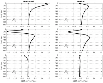
5.2.1 Love Number Partial Derivatives . . . 148
5.2.2 Load Green’s Function Partial Derivatives . . . 152
6 The Sensitivity of Surface Mass Loading Displacement Response to Perturba-tions in the Elastic Structure of the Crust and Mantle 154 6.1 Abstract . . . 154
6.2 Introduction . . . 155
6.3 Methodology . . . 159
6.4 Results . . . 167
6.4.1 Love Number Sensitivities . . . 167
6.4.2 Load Green’s Function Sensitivities . . . 174
6.4.3 Predicted OTL-Induced Surface Displacements . . . 180
6.5 Discussion . . . 199
6.6 Summary and Conclusions . . . 209
6.7 Acknowledgments . . . 210
7 Observations of Ocean Tidal Load Response in South America from Sub-daily GPS Positions 211 7.1 Abstract . . . 211
7.2 Introduction . . . 212
7.3 Predictions . . . 217
7.3.1 Ocean Tide Model Comparisons . . . 221
7.3.2 SNREI Earth Model Comparisons . . . 227
7.4.1 Kinematic GPS Processing . . . 233
7.4.2 Harmonic Analysis . . . 235
7.4.3 Residuals . . . 237
7.4.4 Uncertainty Estimates . . . 241
7.5 Discussion . . . 248
7.6 Summary & Conclusions . . . 260
7.7 Acknowledgments . . . 261
7.8 Appendix A: Process Noise Settings for GPS Analysis . . . 261
7.9 Appendix B: Harmonic Analysis Procedure . . . 268
8 Some Remarks on Surface Mass Loading from Non-OTL Sources 272 8.1 Introduction . . . 272
8.2 Atmospheric Loading . . . 273
8.3 Non-Tidal Ocean Loading . . . 276
8.4 Hydrological Loading . . . 283
9 Summary and Future Directions 290 A Earth Models 293 B Ocean Tide Models 297 B.1 Global Ocean Tide Models . . . 298
B.2 Local Ocean Tide Models . . . 300
B.3 Quality Assessment . . . 300
C Love Number and Green’s Function Tables 302 D Partial Derivatives of Love Numbers 334 E GPS Station Network 352 F Supplemental GPS Theory 359 F.1 Carrier Wave Signals and Satellite Orbits . . . 359
F.2 Pseudorange and Carrier Phase Observables . . . 361
F.3 Ambiguity Resolution, Cycle Slips, and Multipath . . . 362
F.4 Reference Frame Considerations . . . 363
List of Figures
1.1 Tidal forces from a two-body system . . . 4
1.2 Tidal tractive forces . . . 7
1.3 Geometry for deriving the gravitational potential . . . 9
1.4 Tidal amplitude spectra . . . 27
4.1 Load Green’s functions in the CE, CM, and CF reference frames for PREM 131 6.1 Partial derivatives of degree-2 load Love numbers derived from PREM . . . 168
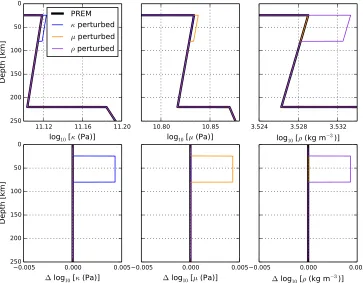
6.2 Partial derivatives of degree-100 load Love numbers derived from PREM . 169 6.3 Partial derivatives of degree-10000 load Love numbers derived from PREM 170 6.4 Earth models derived from perturbations to PREM in the mantle . . . 181
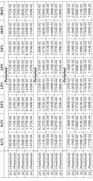
6.5 Differences between load Green’s functions derived from perturbed PREM models . . . 182
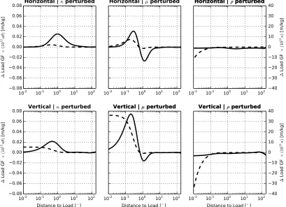
6.6 Sensitivity of displacement load Green’s functions to systematic perturba-tions to the distinct regions of PREM . . . 183
6.7 Sensitivity of displacement load Green’s functions to systematic perturba-tions to 20-km-thick spherical shells in the crust and upper mantle . . . 184
6.8 Sensitivity of displacement load Green’s functions to systematic perturba-tions in crust and upper mantle structure as measured 2.5◦ from the load point . . . 185
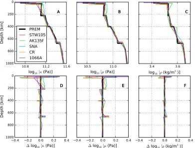
6.9 Comparison between seismologically derived Earth models . . . 186
6.10 Displacement load Green’s functions for various seismologically derived Earth models . . . 187
6.11 Predicted M2OTL-induced surface displacements across Iceland . . . 189
6.12 Vector differences between predicted M2 OTL-induced surface displace-ments derived from PREM and STW105 (Iceland) . . . 190
6.13 Vector differences between predicted M2 OTL-induced surface displace-ments derived from PREM and STW105 (distance to coastline) . . . 191
6.14 Histograms of vector differences between pairs of predicted M2OTL-induced surface displacements for a global grid . . . 192
6.19 Estimated bounds on quadrature errors for the vector differences between
predicted M2OTL-induced displacements . . . 201
6.20 Sensitivity of predicted M2OTL-induced displacements in Iceland (profile A) to perturbations in mantle structure . . . 202
6.21 Sensitivity of predicted M2OTL-induced displacements in Iceland (profile B) to perturbations in mantle structure . . . 203
6.22 Sensitivity of predicted M2OTL-induced displacements in Iceland (profile A) to perturbations in mantle structure (scaled by layer thickness) . . . 204
6.23 Sensitivity of predicted M2OTL-induced displacements in Iceland (profile B) to perturbations in mantle structure (scaled by layer thickness) . . . 205
7.1 Global maps of tide amplitude for the M2, O1, and Mfharmonics . . . 216
7.2 Differences in tide amplitude for the M2, O1, and Mfharmonics . . . 220
7.3 Sensitivity of Earth response to ocean tide models . . . 222
7.4 Sensitivity of Earth response to ocean tide models (mean removed) . . . 223
7.5 Sensitivity of Earth response to ocean tide models (RMS) . . . 225
7.6 Earth model parameters and discrepancies . . . 228
7.7 Displacement load Green’s functions . . . 229
7.8 Sensitivity of Earth response to SNREI Earth models . . . 230
7.9 Sensitivity of Earth response to SNREI Earth models (RMS) . . . 231
7.10 GPS data, harmonic fit, and residuals for station RIO2 . . . 236
7.11 Seismic tomography profile through the Amazonian craton . . . 239
7.12 Observed and predicted OTL-induced surface displacements in South Amer-ica . . . 240
7.13 Periodogram of time series residuals at station RIO2 . . . 242
7.14 Residual M2OTL-induced surface displacements in South America . . . . 245
7.15 Residual O1 OTL-induced surface displacements in South America . . . 246
7.16 Residual Mf OTL-induced surface displacements in South America . . . . 247
7.17 Residual OTL-induced surface displacements shown as vectors . . . 249
7.18 Residual OTL-induced surface displacements shown as vectors (common-mode removed) . . . 250
7.19 Uncertainties in observed OTL-induced surface displacements in South Amer-ica . . . 251
7.20 Residual OTL-induced surface displacements in South America: Compari-son of ocean tide models . . . 252
7.21 Residual OTL-induced surface displacements in South America: Compari-son of SNREI Earth models . . . 253
7.23 Effect of reference frame in the generation of ocean tide models from
satel-lite altimetry data . . . 257
7.24 Recovery of GPS synthetic signals using various coordinate process noise settings . . . 266
7.25 Recovery of GPS synthetic signals using various tropospheric process noise settings . . . 267
8.1 Atmospheric surface pressure anomaly in 2007 . . . 274
8.2 Pressure exerted by the M2, O1, and Mf ocean tides . . . 277
8.3 Modeled displacement response at station TERS due to atmospheric loading 278 8.4 Modeled displacement response at station AC34 due to atmospheric loading 279 8.5 Modeled displacement response at station RIO2 due to atmospheric loading 280 8.6 Validation of ATML and NTOL modeling with Williams and Penna (2011) 281 8.7 Comparison with Williams and Penna (2011) using GPS positions com-puted locally . . . 282
8.8 Non-tidal ocean pressure anomaly in 2007 . . . 284
8.9 Modeled displacement response at station TERS due to non-tidal ocean loading . . . 285
8.10 Modeled displacement response at station AC34 due to non-tidal ocean loading . . . 286
8.11 Modeled displacement response at station RIO2 due to non-tidal ocean loading . . . 287
8.12 Modeled displacement response at station TERS due to a combination of atmospheric and non-tidal ocean loading . . . 288
A.1 Depth profiles of standard SNREI Earth models . . . 294
B.1 M2tide amplitude from FES2012 . . . 299
C.1 Potential Love numbers for several SNREI Earth models . . . 304
C.2 Load Love numbers for several SNREI Earth models . . . 305
C.3 Shear Love numbers for several SNREI Earth models . . . 306
C.4 Stress Love numbers for several SNREI Earth models . . . 307
C.5 Displacement load Green’s functions for several SNREI Earth models in the CM and CE reference frames . . . 308
D.1 Partial derivatives of degree-1 load Love numbers from PREM . . . 335
D.2 Partial derivatives of degree-1 stress Love numbers from PREM . . . 336
D.3 Partial derivatives of degree-2 potential Love numbers from PREM . . . 337
D.4 Partial derivatives of degree-2 load Love numbers from PREM . . . 338
D.5 Partial derivatives of degree-2 shear Love numbers from PREM . . . 339
D.6 Partial derivatives of degree-2 potential Love numbers from 1066A . . . 340
D.8 Partial derivatives of degree-2 shear Love numbers from 1066A . . . 342
D.9 Partial derivatives of degree-3 load Love numbers from PREM . . . 343
D.10 Partial derivatives of degree-4 load Love numbers from PREM . . . 344
D.11 Partial derivatives of degree-10 load Love numbers from PREM . . . 345
D.12 Partial derivatives of degree-100 load Love numbers from PREM . . . 346
D.13 Partial derivatives of degree-1000 load Love numbers from PREM . . . 347
D.14 Partial derivatives of degree-10000 load Love numbers from PREM . . . . 348
D.15 Partial derivatives of degree-2 potential Love numbers for a homogeneous sphere . . . 349
D.16 Partial derivatives of degree-2 load Love numbers for a homogeneous sphere 350 D.17 Partial derivatives of degree-2 shear Love numbers for a homogeneous sphere351 E.1 GPS station activity timeline: 1 . . . 355
E.2 GPS station activity timeline: 2 . . . 356
E.3 GPS station activity timeline: 3 . . . 357
List of Tables
1.1 Doodson’s geodetic coefficients . . . 14
1.2 Astronomical ephemeris for the Earth-moon-sun system . . . 16
1.3 Angular speeds and frequencies of fundamental astronomical parameters: 1 20 1.4 Angular speeds and frequencies of fundamental astronomical parameters: 2 22 1.5 Dominant tidal harmonics . . . 24
2.1 Harmonic-modulation corrections for several dominant tidal harmonics . . 37
2.2 Primary and subsidiary harmonics from the L2 tidal harmonic . . . 43
2.3 Shallow-water harmonics . . . 49
4.1 Surface boundary conditions used to derive Love numbers . . . 116
5.1 A comparison of direct differences between degree-2 load Love numbers derived from perturbations to a homogeneous sphere . . . 153
6.1 Surface boundary conditions and Love number definitions . . . 171
6.2 Comparison of degree-2 load Love number partial derivatives . . . 173
6.3 Degree-2 potential Love numbers . . . 174
7.1 Sensitivity of Earth response to ocean tide models (RMS) . . . 226
7.2 Sensitivity of Earth response to SNREI Earth models (RMS) . . . 227
7.3 Residual OTL-induced surface displacements in South America (RMS) . . 241
7.4 Uncertainties in observed OTL-induced displacements in South America . . 244
A.1 Earth model SNA . . . 295
A.2 Earth model CR . . . 296
C.1 Love numbers for Earth model 1066A . . . 309
C.2 Love numbers for Earth model PREM . . . 310
C.3 Love numbers for Earth model AK135f . . . 311
C.4 Love numbers for a homogeneous sphere . . . 312
C.5 Displacement load Green’s functions for Earth model 1066A . . . 313
C.6 Displacement load Green’s functions for Earth model PREM . . . 316
C.7 Displacement load Green’s functions for Earth model STW105 . . . 319
C.8 Displacement load Green’s functions for Earth model AK135f . . . 322
C.9 Displacement load Green’s functions for Earth model SNA . . . 325
C.10 Displacement load Green’s functions for Earth model CR . . . 328
C.11 Displacement load Green’s functions for a homogeneous sphere . . . 331
1
Tidal Theory
1.1 Introduction and Motivation
Gravitational forcing by the moon and sun deforms the solid Earth both directly through the gravitational potential (body tides) and indirectly through loading by the periodic re-distribution of Earth’s oceans (load tides). Ocean tidal loading (OTL) refers to the process by which tidally redistributed seawater exerts a normal force on Earth’s surface. The mate-rial properties of the crust and upper mantle govern the flexural response of the solid Earth to the weight of the additional water; thus, the OTL response signal, contained within all geodetic measurements, may be exploited to explore Earth’s interior structure.
Whereas the spatial distribution of the body-tide response generally follows that of the equi-librium tide derived directly from the gravitational potential, ocean tides exhibit a complex spatial pattern due to interactions with continental boundaries and bathymetry (Jentzsch, 1997). Thus, whereas body tides are long wavelength phenomena that sample a very large-scale average of Earth structure (e.g., Farrell, 1972a; Latychev et al., 2009), ocean tidal loads are shorter wavelength features that probe Earth’s material properties at finer spatial scales (e.g., Farrell, 1972a; Baker, 1984; Ito & Simons, 2011; Agnew, 2015; Bos et al., 2015). Constraints on Earth’s interior properties derived from surface mass loading (SML) provide an independent means of testing scaling laws and assumptions commonly adopted in seismology, rejecting existing proposed Earth models that are inconsistent with the geodetic observations (e.g., Ito & Simons, 2011; Bos et al., 2015), and addressing out-standing questions in geophysics, such as the long-term stability of continental cratons against tectonic deformation (e.g., Jordan, 1978).
implement the theory using gravity, strain and tilt measurements were limited in effective-ness due to insufficient spatial coverage and high sensitivities to local variations in mate-rial properties (Baker, 1984; Agnew, 2015). Modern Global Navigation Satellite System (GNSS) receivers do not suffer from the same sparsity or sensitivity constraints and record Earth’s response to OTL with sub-millimeter precision (e.g., Penna et al., 2015). Given the precision of modern GNSS observations (Blewitt, 2015), the rapid expansion of global and regional GNSS networks, and the accuracy of contemporary ocean-tide models (Stam-mer et al., 2014), the possibility of using observed OTL-induced surface displacements to investigate Earth’s interior structure has become increasingly tractable.
1.2 Tide-Generating Forces
According to Newton’s law of universal gravitation, the force of gravity,Fg, on a test mass,
m, is given by:
Fg=
G M m
R2 , (1.1)
whereGis the universal gravitational constant,M is the mass of the reference body, andR
is the distance between the center of mass of the reference body and the center of mass of the test body.
Taking the sun as a reference body and the Earth as a test body, followed by the moon as a reference body and the Earth again as a test body, demonstrates that the gravitational force of the sun on the Earth is about 178 times greater than the gravitational force of the moon on the Earth. Thus, although the moon orbits the Earth, the Earth-moon system orbits the sun.
The moon, on the other hand, generates tidal disturbances that are more than twice as large as those due to the sun. Since the tides are created by gravitational forcing, and the sun exerts a greater gravitational pull on the Earth, the relatively large lunar tides might seem counterintuitive.
The key to resolving the apparent discrepancy lies in the definition of the tides as the peri-odic rise and fall in sea level (or deformation of the solid Earth) that results from differential, or unbalanced, gravitational forces throughout the Earth (e.g., Doodson & Warburg, 1941, Sec. 2.2). The differential forces arise because the Earth has a finite diameter over which the gravitational forces are distributed. In other words, the unequal distances between various points on and in the Earth with respect to the external attracting body lead to an unbalanced response to the gravitational forcing.
To Moon A
C
B
D
Figure 1.1: Schematic diagram depicting tidal forces, or accelerations, generated by a two-body system. For the Earth-Moon system, the largest arrows represent an acceleration of 1.14µm s−2. The elliptical outline illustrates a tide-generated equipotential surface (greatly exaggerated). The points A–D, indicated by the dashed lines, are referred to within the text. The diagram has been reproduced and modified with permission from Agnew (2015).
the surface of the Earth, and always directed away from the moon (e.g., Godin, 1972; Pugh, 1987; Pugh & Woodworth, 2014).
The centrifugal force due to revolution about the barycenter is perfectly balanced at the Earth’s center of mass by the gravitational force due to the moon. At other locations in and on the Earth, however, the gravitational force varies, but the centrifugal force remains the same, thereby giving rise to differential forces. Fig. 1.1 illustrates the tidal forces generated by a two-body system.
Since the centrifugal force balances the lunar gravitational force at the center of mass of the Earth, the equation for the centrifugal force on a test mass,m, is given by (e.g., Pugh & Woodworth, 2014, Sec. 3.1):
Fcentrifugal=
G MLm
R2LE , (1.2)
would instead be given by (e.g., Pugh & Woodworth, 2014):
FgA =
G MLm
(RLE−a)2
, (1.3)
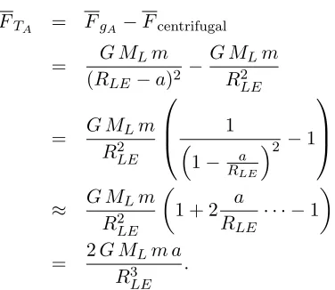
whereais the radius of the Earth (assumed spherical). The difference between the gravita-tional and centrifugal forces yields the tide-generating force,FTA, at point A:
FTA = FgA−Fcentrifugal (1.4)
60 (e.g., Pugh & Woodworth, 2014), I have only kept the first non-zero term in the expansion. Repeating the procedure for point B in Fig. 1.1 yields a vector of the same magnitude, but pointed in the opposite direction (i.e., away from the moon), which generates the familiar tidal bulges.
To examine what happens at the poles, I decompose the tidal forces, or tide-generating forces, into radial and tangential components relative to Earth’s surface (e.g., Doodson & Warburg, 1941). Since RLE is approximately equal toRLC, where RLC is the distance between point C and the center of mass of the moon, the tangential components of the force vectors effectively cancel. The unit vector situated at point C and directed along the path
RLC, however, also has a small surface-normal component, which is approximately equal to− a
RLE (e.g., Doodson & Warburg, 1941, Sec. 2.3). Thus, the tidal force at point C in
Fig. 1.1 is given approximately by:
FTC =−
G MLm a
Analogously,FTD is equivalent in magnitude but opposite in direction toFTC.
It turns out that the components of the tidal forces directed tangential to the surface, other-wise known as the tidaltractiveforces (e.g., Doodson & Warburg, 1941), are principally responsible for generating the tides (e.g., Doodson & Warburg, 1941; Boon, 2004). Com-puting the radial component of the force helps to elucidate this point. In particular, I exam-ine the gravitational force due to the moon versus the gravitational force due to the Earth on a test mass at point A. The gravitational force due to the Earth is given by
FE =
G MEm
a2 (1.6)
and the gravitational force due to the moon is given by
FL=
G MLm
RLA2 , (1.7)
whereRLAis the distance between point A and the center of mass of the moon. The force due to the moon relative to the force due to the Earth is therefore:
FL=
MLa2
MER2LA
To Moon
Figure 1.2: The surface-tangential components of the tidal force vectors resolved onto Earth’s surface. The so-called tractive forces are unopposed by Earth’s gravity and therefore principally responsible for generating the tidal response.
1.3 Tidal Potential
Computing the tide-generating forces is worthwhile for gaining some physical intuition about tides, but for more complete analyses of the tidal spectrum, deriving the tidal poten-tial is preferable. The tidal potenpoten-tial is a scalar, rather than a vector, quantity and hence much easier to develop in computations. The gravitational potential at a point, P, on the Earth’s surface due to the gravitational influence of an external body may be written as (e.g., Doodson, 1921; Melchior, 1983; Pugh & Woodworth, 2014, Sec. 3.2.1):
V = G M
r , (1.9)
Using the geometry shown in Fig. 1.3, I apply the law of cosines to obtain a formula forr:
r2 =a2+R2−2aRcosθ (1.10)
and use this to re-write the equation for the potential:
V = GM
The bracketed term is a generating function for Legendre polynomials (e.g., Boas, 1983, Sec. 12.5). Thus, the potential may be expanded as:
V = GM
where Pn(cosθ) are the Legendre polynomials. The first few Legendre polynomials are (e.g., Boas, 1983; Pugh & Woodworth, 2014):
P0(cosθ) = 1
The first term in Eq. 1.12 is constant-valued and does not generate a force. The second term represents a uniform force in the direction ofOC, and therefore does not generate a tidal ef-fect. The third term, in contrast, produces the largest tidal effect (e.g., Pugh & Woodworth, 2014). Higher-degree terms (beyond the third term) are sometimes neglected, since the po-tential is proportional to Ran, wherenrepresents the spherical harmonic degree (Pugh & Woodworth, 2014). For the moon,Ra ≈ 1
60, and for the sun,
a
R ≈4.3×10
−5. Contributions
O
a
R
θ
r
P
C
Earth
Body 2
Figure 1.3: Schematic diagram depicting the geometry used to construct the gravitational potential observed at point P on the Earth due to the gravitational forcing imposed by a secondary body, “Body 2.” Body 2 is typically the moon or sun, but may be any external body, such as another planet.
magnitude of the potential drops off as RMn+1, it is not necessary to expand the potential for the sun to as high of a degree as for the moon. In the case of the second-degree expansion, for example, MS
R3
S
= 0.46ML
R3
L, where
MS is the mass of the sun, ML is the mass of the moon, andRSandRLare the distances between the center of mass of the Earth and the sun and moon, respectively. Furthermore, it is generally not necessary for practical purposes to expand the potential for either body beyond the third- or fourth-degree (e.g., Cartwright & Taylor, 1971).
Focusing on the degree-2 expansion, the tide-generating potential,VT, may be written as:
VT =
1
2GM
a2 R3(3 cos
2θ−1). (1.13)
the meridian of point P and the meridian of the sub-lunar point. The spherical trigonomet-ric formula relating these quantities is (e.g., Doodson, 1921; Doodson & Warburg, 1941; Schureman, 1971; Pugh & Woodworth, 2014):
cosθ= sinφPsindL+ cosφP cosdLcosCL. (1.14) As such,
cos2θ = sin2φPsin2dL+ cos2φPcos2dLcos2CL+
2 sinφP sindLcosφP cosdLcosCL. (1.15)
Using the trigonometric identity
sin 2u= 2 sinucosu, (1.16)
Eq. 1.15 simplifies to:
cos2θ = sin2φPsin2dL+ cos2φPcos2dLcos2CL+
1
2sin 2φPsin 2dLcosCL. (1.17)
To reduce the order of terms incosCL, I use
cos2CL=
1
2(cos 2CL+ 1) (1.18)
to re-arrange Eq. 1.17, which results in:
cos2θ = sin2φPsin2dL+ cos2φP cos2dL
1
2(cos 2CL+ 1)
+
1
2sin 2φPsin 2dLcosCL, = sin2φPsin2dL+
1 2cos
2φ
Pcos2dLcos 2CL+
1 2cos
2φ
Pcos2dL+
1
Following (Pugh & Woodworth, 2014), the trigonometric identity
cos2u= 1−sin2u (1.20)
may be used to re-write Eq. 1.19 as:
cos2θ = sin2φPsin2dL+
Eq. 1.21 can then be substituted into Eq. 1.13 to obtain a formula for the lunar tide-generating potential, VL, in terms of the astronomical ephemeris (e.g., Doodson, 1921; Pugh, 1987; Pugh & Woodworth, 2014):
VL = whereMLis the mass of the moon and I have made use of the relationship
G= ga
2
ME
whereMEis the mass of the Earth andgis the gravitational acceleration at Earth’s surface. This formulation provides the foundation for a development of the equilibrium tide, which is equivalent to the tidal equipotential on a perfectly rigid Earth (e.g., Agnew, 2015). Note, however, that Eq. 1.22 is only of second-degree (i.e., spherical harmonic degreen = 2), though for practical purposes the potential is typically expanded to at least the third- or fourth-degree for the moon and at least second- or third-degree for the sun (e.g., Cartwright & Taylor, 1971; Cartwright & Edden, 1973; Hartmann & Wenzel, 1995).
Furthermore, Eq. 1.22 does not account for the flattening of the Earth due to rotation or other distortions of the geoid (e.g., Cartwright & Taylor, 1971). Accounting for the shape of the geoid introduces higher-order terms into the development of the tidal potential (e.g., Hartmann & Wenzel, 1995; Roosbeek, 1996, Sec. 4.5), but the effect is apparently small: ∼1.8 ngal for lunar tidal gravity (Roosbeek, 1996). The tidal potential catalogues devel-oped by Doodson (1921), Cartwright & Taylor (1971), and Cartwright & Edden (1973), for example, were not adjusted to account for the secondary effects that arise due to the non-spherical shape of the geoid.
1.4 Equilibrium Tide Formulation
1.4.1 Direct Mathematical Approach
Much of the following development has been reproduced from Pugh (1987) and Pugh & Woodworth (2014), but may also be found in other sources dating back to the cardinal works on tidal harmonic analysis by Darwin (1898) and Doodson (1921) in the late 19th and early 20th centuries.
Theequilibrium tide, or the height of an ideal ocean that is in perfect equilibrium with the tidal forcing (assuming negligible self-attraction effects) (e.g., Schureman, 1971, Par. 88), is given by:
ξ = VT
g , (1.24)
and tide-generating forces to the slope of the equilibrium sea surface (Pugh & Woodworth, 2014).
Combining Eq. 1.24 with Eq. 1.22, an expression for the degree-2 equilibrium tide due to the moon may be derived (e.g., Doodson, 1921; Melchior, 1983; Pugh & Woodworth, 2014, Sec. 3.2.2):
Eq. 1.25 expresses the equilibrium tide in terms of the north latitude of the observation point P (φP) and three time-dependent coefficients, which vary with lunar declination (dL), the distance between the center of mass of the Earth and moon (RL), and the lunar hour angle (CL).
For clarity, a general geodetic factor,G∗, may be defined:
G∗ = 3
whereMLis the mass of the moon,MEis the mass of Earth,gis the mean acceleration due to gravity at Earth’s surface,ais the radius of the Earth (assumed spherical), and 1c is the mean value of R1
L (e.g., Doodson, 1921; Melchior, 1983). Dropping the time-dependent
notation and multiplying by g to convert tidal height back to gravitational potential, Eq. 1.25 may be re-written as (Doodson, 1921):
Doodson’s Geodetic Coefficients
Symbol Formula
Second Degree(n= 2)
G∗0 12G∗(1−3 sin2φP)
G∗1 G∗ sin(2φP)
G∗2 G∗ cos2φ
P
Third Degree(n= 3)
G∗00 1.11803G∗ sinφP(3−5 sin2φP)
G∗01 0.72618G∗ cosφP(1−5 sin2φP)
G∗02 2.59808G∗ sinφP cos2φP
G∗03 G∗ cos3φP
Fourth Degree(n= 4)
G∗000 0.12500G∗(3−30 sin2φP + 35 sin4φP)
G∗001 0.47346G∗ sin(2φP) (3−7 sin2φP)
G∗002 0.77778G∗ cos2φP(1−7 sin2φP)
G∗003 3.07920G∗ sinφP cos3φP
G∗004 G∗ cos4φP
Table 1.1: The general geodetic factor G∗ = 34a g ML
ME
a3
c3, where ML is the mass of the moon,ME is the mass of Earth,gis the mean acceleration due to gravity at Earth’s surface,
ais the radius of Earth (assumed spherical), and 1c is the mean value of R1
L. The numerical
coefficients that precedeG∗in the third- and fourth-degree coefficients are derived from the quantity ac, which is approximately equivalent to the sine of the mean equatorial horizontal parallax (Doodson, 1921).
where
H0 =
2
3−2 sin
2d
L (1.31)
H1 = sin 2dL cosCL (1.32)
H2 = cos2dL cos 2CL, (1.33)
andG∗0,G∗1, andG∗2are Doodson’sGeodetic Coefficients, defined in Table 1.1.
Additional details regarding the expansion of the equilibrium tide may be found in, e.g., Cartwright & Taylor (1971); Doodson (1921); Doodson & Warburg (1941), Ch. 4; Godin (1972), pg. 16-27 and Appendix 1; Pugh (1987), Chs. 3 and 4; and Pugh & Woodworth (2014). Note that, for solar terms,G∗S = 0.46 G∗. A short discussion of equilibrium tide catalogues will be provided later in this chapter (Sec. 1.5).
that each coefficient depends on the lunar hour angle as a cosine term with a different frequency: theC2(t)coefficient includes acos(2CL(t))term, theC1(t)coefficient includes acos(CL(t))term, and theC0(t)coefficient does not include a cosine term with dependence on the hour angle. The response of the equilibrium tide to astronomical forcing is separated into these three coefficients, which vary in spherical harmonic mode as a result of their dependence on the hour angle (e.g., Pugh & Woodworth, 2014).
Tides that do not depend on the hour angle (i.e., coefficient C0(t)) are known as
long-period tides and are characterized by a zonal spherical harmonic function (i.e., n = 2,
m = 0, where m is the spherical harmonic order) (e.g., Melchior, 1983, Ch. 1). Tidal signals proportional tocos(CL(t))(i.e.,C1(t)), characterized by a frequency of one cycle per day, are known asdiurnaltides and are represented by atesseralspherical harmonic function (i.e., n = 2, m = 1). Tidal signals proportional to cos(2CL(t)) (i.e., C2(t)), characterized by a frequency of two cycles per day, are known assemidiurnaltides and are represented by asectorialspherical harmonic function (i.e.,n= 2,m= 2).
Note also the dependence of the coefficients on lunar declination. From the 32sin2dL(t)−12
portion of theC0(t)term, it is clear that the long-period tides reach a maximum amplitude at the poles and zero amplitude at±35.27◦ declination (e.g., Pugh & Woodworth, 2014, Sec. 3.2.2). TheC1(t)term, which is proportional tosin 2dL(t), also varies at twice the rate of variations in lunar declination, reaching a maximum amplitude at±45◦and a minimum am-plitude at the equator and poles. TheC2(t)term varies withcos2dL(t); thus, semidiurnal tides reach a maximum amplitude at the equator and zero amplitude at the poles.
Similarly, the equilibrium tide depends on the latitude (positive north) of the observation point, φP. The long-period tides, proportional tosin2φP, reach maximum values at the poles. The diurnal tides, proportional to sin 2φP, are maximized at ±45◦ latitude. The semidiurnal tides, proportional tocos2φP, are maximized at the equator.
Parameter Description Symbol Temporal Evolution
Lunar Hour Angle (radians) CL λP + (ω0+ω3)t−π−AL Solar Hour Angle (radians) CS λP + (ω0+ω3)t−π−AS Mean longitude of moon (◦) s 277.02 + 481267.89T + 0.0011T2
Mean longitude of sun (◦) h 280.19 + 36000.77T+ 0.0003T2
Longitude of lunar perigee (◦) p 334.39 + 4069.04T−0.0103T2 Longitude of lunar ascending node (◦) N 259.16−1934.14T+ 0.0021T2 Longitude of perihelion (◦) p0 281.22 + 1.72T+ 0.0005T2
Spatiotemporal Variables
Time in Julian centuries T 365(Y−1900)+(36525D−1)+i+HM S
Current year Y
Current day D
Current hour, minute, second HM S units of days
Leap year correction i integer part of (Y-1901)/4
East longitude of observation point P λP units of radians
Sidereal time at Greenwich Meridian t measured from First Point of Aries Right Ascension of Moon/Sun AL/AS see text for equations
Table 1.2: Astronomical parameters used to describe the temporal variations of the moon and sun relative to the Earth (e.g., Pugh, 1987). Only six of the seven parameters listed are independent. The variables ω0 and ω3 represent angular speeds of the astronomical parameters, which are listed in Table 1.3. See also, e.g., Doodson (1921), Doodson & Warburg (1941), Schureman (1971), Melchior (1983), and Meeus (1998).
are replaced withdS,MS, andRS, respectively, wheredSrepresents the solar declination,
MSis the mass of the sun, andRS is the distance between the center of mass of the Earth and the center of mass of the sun. Furthermore, the hour angle,CS, represents the angular separation between the sub-solar point and the observation point, P.
Earth-Sun System: The distance between the Earth and sun,RS, is given by (e.g., Dood-son & Warburg, 1941; Munk & Cartwright, 1966; Pugh, 1987; Pugh & Woodworth, 2014):
RS=
R∗S
1 +eScos(h−p0)
, (1.34)
(solar) parallax, 8.7941500 from Munk & Cartwright (1966), may be related to the mean earth-sun distance by:
6371 km
1 60
8.79415 60
π
180
≈1.5×10⁸km. (1.35)
Additional tabulations of astronomical parameters can be found in Wenzel (1997) and Meeus (1998).
The right ascension for the sun, in equatorial coordinates, is (e.g., Pugh & Woodworth, 2014):
AS=λS−tan2
S
2
sin(2λS), (1.36)
where
λS =h+ 2esin(h−p0) (1.37)
andS is the solar ecliptic latitude, or ≈ 23.452◦ (Munk & Cartwright, 1966). The solar declination in terms of equatorial coordinates is then (e.g., Pugh & Woodworth, 2014):
dS = sin−1(sin(λS) sin(S)). (1.38)
Earth-Moon System: The distance between the Earth and moon,RL, is given by (Pugh, 1987; Pugh & Woodworth, 2014):
RL=
R∗L
1 +eLcos(s−p) +solar perturbations
, (1.39)
whereeLis the eccentricity of the moon’s orbit about the Earth, which varies from 0.044 to 0.067, andR∗Lis the mean lunar distance. The right ascension for the moon is (e.g., Pugh & Woodworth, 2014):
AL=λL−tan2
L
2
sin(2λL), (1.40)
where
λL=s+ 2e sin(s−p) +solar perturbations, (1.41) and
is the lunar ecliptic latitude. The lunar declination is given by:
dL= sin−1(sin(λL) sin(L)). (1.43)
Characteristics of the actual ocean tides turn out to be quite different from the ideal equi-librium tide due to complicated effects related to finite ocean depths, bathymetry, and con-tinental boundaries.
1.4.2 Harmonic Decomposition Approach
Six independent parameters are necessary to describe the temporal variations ofR,d, and
C in the tidal potential for both the sun and moon. After careful consideration, Doodson (1921) selected six astronomical parameters that are well-suited to harmonic analysis and often used in practice (e.g., Foreman, 1977, Sec. 2.1.1):
τ = local mean lunar time,
s = mean longitude of moon,
h = mean longitude of sun,
p = mean longitude of lunar perigee,
N0 = −N, whereN is the mean longitude of lunar ascending node,
p0 = mean longitude of perihelion.
Note thatτ is equivalent toCL when referenced to the same observation point, which is typically set at the Greenwich Meridian. Furthermore, the two parameters have the same angular speed. Alternatively, the mean solar time, t, may be used in place of τ; the two parameters are related by other fundamental astronomical parameters:τ =t−s+h(e.g., Doodson, 1921).
The expression for the equilibrium tide may now be expanded into a series of harmonic terms. For example, I make use of Eq. 1.39 and Doodson’s astronomical parameters to re-write Eq. 1.28 as (e.g., Pugh & Woodworth, 2014, Sec. 4.2.1):
C2(t) =
whereeL is the lunar eccentricity and I have kept only the lowest-degree terms. For the full expansion, one would need to substitute expressions for the declination in terms of the astronomical parameters as well. A more complete expansion of the equilibrium tide contains thousands of terms (infinite in a full expansion), but in practice, only a few dom-inant harmonics are essential. Equilibrium tide catalogues, expanded to include hundreds to thousands of tidal harmonics, may be found in the literature (e.g., Cartwright & Taylor, 1971; Cartwright & Edden, 1973; Hartmann & Wenzel, 1995).
Angular Speeds of Astronomical Parameters
Period Frequency Angular Speed
Parameter (days) (cycles/day) Symbol (rad/hour) (◦/hour) Mean solar day 1.00 1.00 C˙S = ˙t ω0 = 0.26 σ0=15.00 Mean lunar day 1.04 9.66E-1 C˙L= ˙τ ω1 = 0.25 σ1=14.49 Sidereal month 27.32 3.66E-2 s˙ ω2 = 9.58E-3 σ2=0.55 Tropical year 365.24 2.74E-3 h˙ ω3 = 7.173E-4 σ3=0.04 Lunar perigee 8.85 (years) 3.09E-4 p˙ ω4 = 8.03E-5 σ4=4.6E-3 Lunar nodal
regression 18.61 (years) 1.47E-4 −N˙ = ˙N0 ω
5 = 3.84E-5 σ5=2.2E-3
Perihelion 20942 (years) - p˙0 ω
6 ≈0 σ6≈0 Table 1.3: Angular speeds, or frequencies, of the astronomical parameters from Table 1.2. The angular speeds, ω, represent the mean rates of change, in radians per hour, of the astronomical parameters:CS,CL,s,h,p,N0,p0. For units of degrees per hour, the angular speeds are denoted byσ. A dot above an astronomical parameter indicates differentiation with respect to time. Since the astronomical parameters vary in time with terms higher than first order, the angular speeds also change with time, albeit slowly (see text for details).
speed of2ω0+ 2ω3−3ω2 +ω4 = 2ω1−ω2 +ω4 = 0.4964rad/hour= 28.4398◦/hour. Furthermore, the third harmonic term in Eq. 1.44, given the name L2, has an angular speed of2ω0+ 2ω3−ω2−ω4 = 2ω1+ω2−ω4 = 0.5154rad/hour= 29.5286◦/hour. Note that the three harmonics differ in amplitude, which is modulated in this case by the lunar orbital eccentricity.
Angular Speed: The general form for the angular speed,ω, of a given tidal harmonic,η, is (e.g., Pugh & Woodworth, 2014, Sec. 2.4.1):
ωη =ηaω1+ηb ω2+ηcω3+ηdω4+ηeω5+ηf ω6, (1.45) whereω1toω6are angular speeds, generally in rad/hour, derived from the lunar and solar ephemera. First-order approximations of the angular speeds are provided in Table 1.3. More precise values may be obtained by taking the first time derivatives of the astronomical parameters (Table 1.2). The coefficients ηa to ηf are small integer values that form the
Doodson number for harmonic η. Distinct sets of integer coefficients (ηa through ηf) are used to determine unique sums and differences of the astronomical frequencies, which represent individual tidal harmonics in the expansion of the equilibrium tide (e.g., Doodson & Warburg, 1941; Pugh & Woodworth, 2014).
The M2harmonic, for example, has a Doodson number of [2 0 0 0 0 0]; thus, the M2tide has a frequency ofωM2 = 2ω1+ 0ω2+ 0ω3+... = 0.5059rad/hour = 28.9842
◦/hour.
Note that it is not necessary to include ω0, sinceω0 may be written in terms of other as-tronomical frequencies (i.e., ω0 = ω1+ω2−ω3). For a degree-2 expansion of the tidal potential, the coefficientηa may only be 0, 1, or 2, representing the long-period, diurnal, and semidiurnal tidal species, respectively (e.g., Pugh & Woodworth, 2014, Sec. 4.2.1). The value of coefficientηbdefines the tidalgroupand the value of coefficientηcdefines the tidalconstituent. Coefficientsηb throughηf generally range from -5 to +5. Values greater than two for coefficientηarepresent species at frequencies higher than semidiurnal, such as terdiurnal tides (ηa= 3), that arise from higher-order expansions of the tidal potential. The full set of six integer coefficients defines a tidalharmonic, also sometimes referred to as a tidalargument.
Astronomical Frequencies to Higher Order
Element Frequency Formula (deg/hour) Symbols
Mean solar day 1∗(360/24) ω0 C˙S = ˙t
Mean lunar day 1 +ω2-ω3 ω1 C˙L= ˙τ
Sidereal month [(481267.89 + 0.0022T)/36525]/24 ω2 s˙ Tropical year [(36000.77 + 0.0006T)/36525]/24 ω3 h˙ Lunar perigee [(4069.04−0.0206T)/36525]/24 ω4 p˙
Lunar nodal regression −{[(−1934.14 + 0.0042T)/36525]/24} ω5 N˙0 =−N˙ Perihelion [(1.72 + 0.0010T)/36525]/24 ω6 p˙0
Table 1.4: Astronomical frequencies in general form. The angular speeds, ω, represent the mean rates of change of the astronomical parameters: CS, CL, s, h,p, N0, p0. Time derivates were taken of the astronomical parameters in Table 1.2 to derive the frequency formulae in column 2. Tis in Julian centuries.
only manifest after an expansion to at least the third degree (e.g., Godin, 1972).
To avoid negative numbers in the six-digit set, Doodson added+5to each of the integersηb throughηf. With the arithmetic adjustment to the Doodson number, the angular speed must also be adjusted by subtractingωη = 5ω2+5ω3+5ω4+5ω5+5ω6. Unadjusted Doodson numbers, which include negative values, are also common in the literature (e.g., Cartwright & Taylor, 1971; Godin, 1972). Here, I adopt the unadjusted Doodson-number convention, and therefore eliminate the need to correct for the offset in computing the angular speed (as well as other parameters, such as the astronomical argument, that are discussed later).
Astronomical Argument: Analogous to the angular speed, the astronomical argument may be written as (e.g., Godin, 1972, Sec. 0.4.2):
Vη(t) =ηaτ(t) +ηb s(t) +ηch(t) +ηdp(t) +ηeN0(t) +ηf p0(t). (1.46) The astronomical argument, which may be evaluated using Table 1.2 (and Vη(t) modulo
360◦for large angles), provides the reference phase angle for tidal harmonicηat timet.
1.5 Tidal Potential Catalogues
Tidal potential catalogues, or equilibrium tide catalogues, distill the gravitational inter-actions between the Earth and neighboring astronomical bodies into individual harmonic terms, each with a unique Doodson number and a potential height. Sir G.H. Darwin de-veloped the first tidal potential catalogue of harmonic terms in the late 19th century (Dar-win, 1898). Subsequently, Doodson made great advancements in the theory of tidal har-monic analysis, expanding substantially upon the number of catalogued harhar-monics (Dood-son, 1921). Doodson’s catalogue was used for most of the 20th century until Cartwright & Taylor (1971) and Cartwright & Edden (1973) further expanded and improved the catalogue using modern computer power. Although the Cartwright, Taylor, and Edden catalogue (ab-breviated as the CTE catalogue) is still often used today, additional and yet more extensive catalogues have since been developed. For example, Hartmann & Wenzel (1995) expanded the tidal potential to include nearly 13000 harmonics, with gravitational contributions from the moon and sun as well as from Mercury, Venus, Mars, Jupiter, and Saturn. More on the history of tidal analysis and the development of tidal potential catalogues may be found in Cartwright (1999).
The total tidal potential,VT, is given by:
Dominant Tidal Harmonics
Doodson Number Speed Equilibrium
Constituent ηa ηb ηc ηd ηe ηf σ(◦/hour) f (cycles/day) Amplitude
Z0 0 0 0 0 0 0 0.0000 0.0000 0.73869G∗0
Sa 0 0 1 0 0 -1 0.0411 0.0027 0.01160G∗0
Ssa 0 0 2 0 0 0 0.0821 0.0055 0.07299G∗0
Mm 0 1 0 -1 0 0 0.5444 0.0363 0.08254G∗0
Mf 0 2 0 0 0 0 1.0980 0.0732 0.15642G∗0
2Q1 1 -3 0 2 0 0 12.8543 0.8570 0.00955G∗1
σ1 1 -3 2 0 0 0 12.9271 0.8618 0.01153G∗1
Q1 1 -2 0 1 0 0 13.3987 0.8932 0.07216G∗1
ρ1 1 -2 2 -1 0 0 13.4715 0.8981 0.01371G∗1
O1 1 -1 0 0 0 0 13.9430 0.9295 0.37689G∗1
τ1 1 -1 2 0 0 0 14.0252 0.9350 0.00491G∗1
M1 1 0 0 -1 0 0 14.4874 0.9658 0.01065G∗1
N O1 1 0 0 1 0 0 14.4967 0.9664 0.02964G∗1
χ1 1 0 2 -1 0 0 14.5695 0.9713 0.00566G∗1
π1 1 1 -3 0 0 1 14.9179 0.9945 0.01029G∗1
P1 1 1 -2 0 0 0 14.9589 0.9973 0.17584G∗1
S1 1 1 -1 0 0 1 15.0000 1.0000 0.00423G∗1
K1 1 1 0 0 0 0 15.0411 1.0027 0.53050G∗1
ψ1 1 1 1 0 0 -1 15.0821 1.0055 0.00423G∗1
φ1 1 1 2 0 0 0 15.1232 1.0082 0.00756G∗1
θ1 1 2 -2 1 0 0 15.5126 1.0342 0.00566G∗1
J1 1 2 0 -1 0 0 15.5854 1.0390 0.02964G∗1
OO1 1 3 0 0 0 0 16.1391 1.0759 0.01623G∗1
2 2 -3 2 1 0 0 27.4238 1.8283 0.00671G∗2
2N2 2 -2 0 2 0 0 27.8954 1.8597 0.02301G∗2
µ2 2 -2 2 0 0 0 27.9682 1.8645 0.02777G∗2
N2 2 -1 0 1 0 0 28.4397 1.8960 0.17387G∗2
ν2 2 -1 2 -1 0 0 28.5126 1.9008 0.03303G∗2
M2 2 0 0 0 0 0 28.9841 1.9322 0.90812G∗2
λ2 2 1 -2 1 0 0 29.4556 1.9637 0.00670G∗2
L2 2 1 0 -1 0 0 29.5285 1.9686 0.02567G∗2
T2 2 2 -3 0 0 1 29.9589 1.9973 0.02479G∗2
S2 2 2 -2 0 0 0 30.0000 2.0000 0.42358G∗2
R2 2 2 -1 0 0 -1 30.0411 2.0027 0.00354G∗2
K2 2 2 0 0 0 0 30.0821 2.0055 0.11506G∗2
η2 2 3 0 -1 0 0 30.6265 2.0418 0.00643G∗2
In terms of the astronomical parameters, the expansion of the tidal potential to spherical harmonic degree-3 may be written as (Godin, 1972):
VT0,2 = for the long-period and semidiurnal tidal harmonics, and:
VT1,3 =
for the diurnal and terdiurnal tidal harmonics. G∗ηa and G∗0ηa are Doodson’s geodetic co-efficients for degree-2 and degree-3 harmonic species (Table 1.1), respectively, (ηaτ +
ηbs+ηch+ηdp+ηeN0 +ηfp0)defines the astronomical argument for harmonicη, and
Aηaηbηcηdηeηf andBηaηbηcηdηeηf represent the (scaled) amplitude coefficients of the
har-monic terms (Godin, 1972). All variables and coefficients are equivalent in Eqs. 1.48 and 1.49, but note the swap of the geodetic coefficients. Also note that, for an expansion up to degree-3 only,G∗3is undefined and all the sine terms will be zero (Godin, 1972; Cartwright & Taylor, 1971).
EitherAorB will be nonzero for a particular tidal harmonic (i.e., for a unique sequence [ηaηbηcηdηeηf]), but not both. Tidal potential catalogues list each unique sequence [ηaηbηcηdηeηf], which is also the Doodson number of each harmonic, along with its cor-responding amplitude coefficient, typically scaled. In Eqs. 1.48 and 1.49, the amplitudes are scaled by Doodson’s geodetic coefficients. In this case, it is simple to convert catalogue amplitudes (given as the A and B coefficient terms) back to actual tidal heights:
Aη =
G∗ηa
and
Bη =
G∗0ηa
g Bηaηbηcηdηeηf. (1.51)
Section 0.4 of Godin (1972) provides more information on the Doodson catalogue scheme. Also note thatG∗S = 0.46G∗, and hence tidal heights derived from solar ephemeris must be adjusted by this constant factor, which is based on the mass ratio between the moon and the sun as well as the ratio of earth-moon distance to earth-sun distance.
Cartwright & Taylor (1971) adopted an alternative approach to Doodson’s lengthy algebraic expansions: they generated the time-dependent, spherical harmonic coefficients directly us-ing the most up-to-date lunar and solar ephemeris and the “response method” of tidal anal-ysis (Munk & Cartwright, 1966). Amplitudes of individual tidal harmonics, shown in Fig. 1.4 using the Doodson scaling convention, were then extracted from the time series using filtering methods. Agnew (2015) reviews this approach. The CTE scaling convention dif-fers from that of Doodson, though the definitions are directly related (Cartwright & Taylor (1971), Table 2).
Regardless of the tidal potential catalogue adopted for a tidal harmonic analysis, making note of the catalogue’s sign convention is important. The most common variation in sign convention occurs with the fifth astronomical parameter pertaining to the regression of the lunar ascending node. Sometimes the fifth astronomical parameter is taken to be the pre-cession of the lunar ascending node,N, but perhaps more commonly, the fifth astronomical parameter is taken to be the regression of the lunar ascending node,N0 =−N. The adopted convention therefore affects the sign of the fifth Doodson coefficient,ηe, as well as the sign ofω5and the astronomical parameter itself. It is simply important to be consistent through-out an analysis, regardless of which convention is assumed.
1.6 Physical Interpretation of Tidal Harmonics
Frequency (cycles/day)
Tidal Harmonic Amplitude Spectra
Darwin, 1898; Pugh & Woodworth, 2014, Sec. 4.2.1). Here, I highlight a few examples that elucidate the origins of some of the most prominent astronomical constituents, beginning with the semidiurnal species.
From Eqs. 1.30 and 1.33, the lunarsemidiurnalequilibrium tide varies as:
cL
RL
3
cos2dL cos 2CL. (1.52)
First, imagine a fictitious body that moves only in the plane of Earth’s equator (i.e.,dL= 0). Next, suppose that the fictitious body moves at the moon’s mean speed and at the moon’s mean distance from Earth (i.e., cL
RL = 1). The two stipulations yield a lunar semidiurnal
tide that is proportional only tocos 2CL, which has a period of half a lunar day, a Doodson number of [2 0 0 0 0 0], and an angular speed of 2ω1. The particular harmonic just de-scribed is the principal lunar semidiurnal tide and, due to its large amplitude and significant presence around the world, has been given a special name: the M2 tidal harmonic (e.g.,
Doodson & Warburg, 1941; Pugh & Woodworth, 2014).
Next, I consider a situation in which the moon remains in the plane of the equator, but the orbital distance of the moon is allowed to vary (i.e.,RL 6= const). This gives rise to, in the first instance, two additional “fictitious” bodies that have angular speeds that differ from that of M2 by the addition and subtraction of the speed of variation in moon-Earth separation distance, RL. The variation in moon-Earth separation distance has a period 27.555 mean solar days, which is nearly but not precisely equivalent to the length of a sidereal month (or the period of revolution of the moon in longitude). In terms of the six fundamental astronomical parameters defined previously, the astronomical argument for this special type of lunar month could be expressed either as (−s+p) or (s−p). Each of these combinations of astronomical parameters yields a period equivalent to that of the period of variation in moon-Earth separation distance (e.g., drawing from Table 1.3, f 1
2−f4 =
1
a fictitious body that orbits Earth with an angular speed of(2ω1+ω2 −ω4) is calledL2
(e.g., Pugh & Woodworth, 2014, Sec. 4.2.1). N2 is also referred to as the larger lunar el-liptic semidiurnal tidal harmonic, whereasL2is also referred to as the smaller lunar elliptic semidiurnal harmonic (e.g., Doodson & Warburg, 1941, Ch. 6).
From Eqs. 1.30 and 1.32, the lunardiurnalequilibrium tide varies as:
cL
RL
3
sin 2dLcosCL. (1.53)
Note that, according to the degree-2 expansion of the equilibrium tide (Eq. 1.30), all diurnal tides generated from fictitious bodies that orbit in the plane of the equator (dL = 0) have zero amplitude. Due to the finite size of the Earth, however, a small diurnal tide,M1, arises even fordL= 0because the tide at the sub-lunar point will be slightly larger than the tide at the antipode. The first three Doodson numbers for the M1constituent cluster are [1 0 0]. Within that cluster, the harmonic with the largest amplitude has a Doodson number of [1 0 0 -1 0 0], which matches the frequency of a prominent shallow-water tide, to be discussed later. The harmonics [1 0 0 0 0 0] and [1 0 0 1 0 0] also make significant contributions to the constituent cluster. The harmonic [1 0 0 0 0 0] has a frequency of14.4921◦ per mean solar hour and represents the difference in tidal heights on opposite sides of Earth for a mean moon, which orbits Earth in the equatorial plane at a mean distance and at mean speed. The harmonics [1 0 0 1 0 0] and [1 0 0 -1 0 0] differ from the harmonic [1 0 0 0 0 0] by the 8.85-year cycle of the longitude of lunar perigee.
The largest diurnal tides occur when the absolute value of(sin 2dL)is maximized, or when
arise by accounting for variations in the moon-Earth separation distance, as for the semidi-urnal tides. Recalling that variations in lunar distance, or lunar parallax, are represented by astronomical arguments of(s−p)or(−s+p), four new harmonics may be readily derived:
[τ +s+ (s−p)],[τ +s+ (−s+p)], [τ −s+ (s−p)], and[τ −s+ (−s+p)]. The first has an angular speed of14.4921 + 0.5490 + 0.5490−0.0046 = 15.5855◦ per mean solar hour and has been given the special name ofJ1 (e.g., Pugh & Woodworth, 2014, Sec. 4.2.1). The second and third are simply [1 0 0 1 0 0] and [1 0 0 -1 0 0], which are harmonics within the M1 constituent cluster as mentioned previously. The fourth,Q1, has an angular speed of14.4921−0.5490−0.5490 + 0.0046 = 13.3987◦per mean solar hour.
The conceptual key to understanding diurnal tides is visualizing a tidal bulge that is inclined relative to the equator (Boon, 2004). Thus, as Earth rotates, an observer at a nonzero lati-tude will observe a slightly larger high-tide at one time of day and a slightly lower high-tide approximately half a day later. This difference in the tidal heights may roughly be con-sidered the diurnal tide, though other processes (including contributions from long-period tides) will also play a role.
From Eqs. 1.30 and 1.31, the lunar equilibriumlong-periodtide varies as:
In this case, tidal height does not depend on lunar hour angle, and hence tidal periods of the so-called long-period harmonics are never shorter than one day in length. The first Doodson number, which defines the tidal species, is therefore zero for all long-period harmonic terms. Tides of this nature arise as a consequence of the longer period astronomical parameters, such as the sidereal month and the cycle of lunar perigee.
One of the most important long-period tides is the lunar fortnightly tide,Mf. Noting that
Thus, the period of the declination-dependent term is one-half of the full declinational cycle, or one-half of a sidereal month, which corresponds to an angular speed of2σ2 = 1.0980◦ per mean solar hour and a Doodson number of [0 2 0 0 0 0]. The variation in lunar parallax (or moon-Earth distance), which has an angular speed ofσ2−σ4 = 0.5444◦per mean solar hour, yields the lunar monthly harmonic constituent,Mm, with a period of 27.555 days.
Solar constituents are, of course, derived in much the same way, except that solar parameters are substituted for the lunar parameters (e.g.,RSis substituted forRL,dSis substituted for
dL, andCS is substituted forCL). More information may be found in, e.g., Boon (2004), Ch. 6 of Doodson & Warburg (1941), and Ch. 4 of Pugh & Woodworth (2014).
1.7 Tidal Dynamics
Here, I briefly summarize a few important points related to tidal dynamics. For more elab-orate introductions, the reader may consult, e.g., Doodson & Warburg (1941) or Pugh & Woodworth (2014). The concept of the equilibrium tide does not apply directly to the dy-namic ocean tides observed on Earth. The true ocean tides contend with sharp continental boundaries, bathymetry, Earth rotation, elastic deformation of the sea floor, and frictional interfaces.
Neglecting non-linear effects, the dispersion relation for gravity waves is given by (e.g., Wright et al., 1999):
c=
r
g
ktanh(kH), (1.56)
wherec is the wave speed,g is the gravitational acceleration at Earth’s surface, H is the water depth, andkis the wavenumber. If the water depth is much less than the wavelength,
λ, thentanh(kH) ≈ kH. Thus, the wave speed reduces to (e.g., Doodson & Warburg, 1941; Pugh & Woodworth, 2014):
c=pg H (1.57)
in the so-called “shallow-water approximation,” which well describes tides in the pelagic ocean (e.g., Pugh & Woodworth, 2014). In practice, Eq. 1.57 is assumed to apply when
water depth to tidal wavelength, the amplitude of the tidal wave must also be much smaller than the water depth in order to mitigate non-linear effects (e.g., Parker, 2007; Pugh & Woodworth, 2014). Note thatλ=c T, whereT is the tidal period, and thatω=c k, where
ωis the angular frequency of the tidal wave.
The continental boundaries form ocean basins as well as constricted bays and seas, leading to local resonance effects. In general, the world’s oceans exhibit resonant frequencies near to the semidiurnal tidal frequency, reinforcing the strength and amplitude of the tidal waves (e.g., Pugh & Woodworth, 2014). In some parts of the world, such as the Bay of Fundy, resonant effects generate tidal amplitudes in excess of 10 m (e.g., Pugh & Woodworth, 2014, Sec. 1.3).
the source and the mass (amplitude response) is approximately zero, and the relative phase between the source and the mass (phase response) is also approximately zero.
For Earth’s oceans, the natural period may be estimated as the time required for a wave to propagate a quarter of the Earth’s circumference and back again (Souchay et al., 2012). Assuming that the speed of the wave is given by Eq. 1.57 with no impeding continents, the natural period of Earth’s oceans is approximately equivalent to 30 hours for a water depth of 4 km, which is significantly longer than the semidiurnal tidal period of∼12 hours. In this idealized case, the oceans are generally out-of-phase with respect to the moon and sun at semidiurnal and diurnal periods. To be in-phase with the gravitational forcing, the oceans would need to be significantly deeper (>∼20 km). The solid Earth, in contrast, exhibits a natural period of∼1 hour (derived from Earth’s free oscillations), which is much shorter than the forcing period and therefore more or less in-phase with the gravitational forcing. Recall, however, that the oceans are much more complicated than this simple thought experiment might suggest, largely due to continental boundaries and Earth rotation.
1.8 Suggestions for Further Reading
2
Harmonic Analysis
2.1 Introduction
The forcing function that generates the tides (i.e., the astronomical ephemeris) may be bro-ken down into individual harmonic periods (e.g., Darwin, 1898; Doodson, 1921; Doodson & Warburg, 1941). The total forcing from the combined harmonics excites responses within and on the Earth that are also periodic. Harmonic analysis aims to extract the amplitude and phase of individual tidal harmonics, each with a unique frequency, from a time series of ar-bitrary length. In other words, the tidal signal at a particular location may be represented by the summation of a series of cosine terms. It is worth noting that non-harmonic techniques have also been developed to describe the tidal response, such as the response method (e.g., Munk & Cartwright, 1966; Pugh & Woodworth, 2014).
Formally, a tidal harmonic,η, may be characterized by a harmonic expression of the form (e.g., Pugh & Woodworth, 2014, Sec. 4.2):
Aηcos(σηt−φη), (2.1)
where A is the amplitude, σ is the angular speed in degrees per mean solar hour (σ =
180
π
ω), t is the time in mean solar hours, and φ is the phase lag in degrees measured relative to the start of the time series.
phases are generally referenced to the peak in the equilibrium tide at the equator (e.g., Bos et al., 2000). Thus, an additional term must be included: the astronomical argument,Vη(t0). With the astronomical argument included, the harmonic expression becomes:
Aηcos(Vη(t0) +σηt−φη). (2.2)
Since the angular speed contains higher-order secular terms, the expression may be written more precisely. Rather than evaluating the astronomical argument at the beginning of the time series and assuming a linear relationship in its temporal progression, the astronomical argument may be computed explicitly at every epoch (e.g., Foreman et al., 2009). Formally,
Aηcos(Vη(t)−φη), (2.3)
where
Vη(t)∼Vη(t0) +σηt. (2.4) Time series of tidal data contain many individual harmonics, some of which may be very close in the frequency domain. If two harmonics are not separable in frequency over the length of the time series, then the smaller amplitude harmonic will modulate the amplitude and phase of the larger amplitude harmonic over time. Given a time series less than 18.6 years in length, for example, two tidal harmonics separated by one cycle in the regression of the lunar ascending node will not be resolvable. Attempts to extract the amplitude and phase of one of the harmonics, however, will be contaminated by the other harmonic. Thus, correction factors are introduced to account for the modulations introduced by the sub-sidiary harmonics in the frequency domain (e.g., Doodson, 1924a; Doodson & Warburg, 1941; Godin, 1972; Pugh & Woodworth, 2014):
are separated from a primary harmonic by integer cycles in the lunar ascending node, the harmonic-modulation correction factors are referred to asnodal modulations(e.g., Pugh & Woodworth, 2014). Since modulations also occur due to harmonic separations in other astronomical cycles, such as lunar perigee, the modulations have also been more generally referred to assatellite modulations(Foreman et al., 2009). The nomenclature ofsatellite modulations, however, may cause confusion with modern space-based geodesy platforms; thus, I refer to the modulations in a generic sense asharmonic modulations.
Traditionally, to save on computational resources, tidal analyses have applied harmonic-modulation correction factors after an initial least squares fit to the time series (e.g., Godin, 1972; Pawlowicz et al., 2002). Accounting for the harmonic modulations a posteriori often involves the application of constant correction factors that may be assumed constant only over short time windows, such as one year of data or less (e.g., Schureman, 1971, Par. 346). Correcting for the harmonic modulations at the post-processing stage and thereby limiting an analysis to a short time span of data are unnecessary sacrifices with modern computa-tional resources (Foreman et al., 2009). Updating the harmonic-modulation corrections, as well as the astronomical argument, at every epoch in the time series allows for seamless processing of multiple years of data in a single estimation step.
2.2 Harmonic Modulations and Corrections
Recall that a tidal constituent represents a cluster of tidal harmonics that share the same first three coefficients in a Doodson number (i.e.,ηa,ηb, andηc). The harmonic with the largest amplitude from the tidal potential catalogue is typically taken to be the primary, or domi-nant, harmonic. Additional harmonics within the same constituent cluster are referred to as
Harmonic Modulations
Constituent