Bringing Order to Chaos: A Non Sequential Approach for Browsing Large Sets of Found Audio Data

Bringing Order to Chaos: A Non-Sequential Approach for Browsing Large Sets

of Found Audio Data

Per Fallgren, Zofia Malisz, Jens Edlund

[email protected], [email protected], [email protected]

Abstract

We present a novel and general approach for fast and efficient non-sequential browsing of sound in large archives that we know little or nothing about, e.g. so calledfound data– data not recorded with the specific purpose to be analysed or used as training data. Our main motivation is to address some of the problems speech and speech technology researchers see when they try to capitalise on the huge quantities of speech data that reside in public archives. Our method is a combination of audio browsing through massively multi-object sound environments and a well-known unsupervised dimensionality reduction algorithm (SOM). We test the process chain on four data sets of different nature (speech, speech and music, farm animals, and farm animals mixed with farm sounds). The methods are shown to combine well, resulting in rapid and readily interpretable observations. Finally, our initial results are demonstrated in prototype software which is freely available.

Keywords:found data, data visualisation, speech archives

1.

Introduction

1.1.

Found data for speech technology

The availability of usable data becomes ever more impor-tant as data-driven methods continue to dominate virtually every field. Numerous organisations (e.g. the Wikime-dia Foundation1_{, the World Wide Web Consortium}2_{, and}

the Open Data Institute3_{) push hard for Open Data.}

Al-though language data, and speech data in particular, is rid-dled with complex legally restricting considerations (Ed-lund and Gustafson, 2016) and less likely to be ”non-privacy-restricted” and ”non-confidential” as required of Open Data, the use of data-driven methods in language technology (LT) and speech technology (ST) is nothing less than a modern success story. In the intersection of LT and other fields, such as history and politics, social sciences and health (Gregory and Ell, 2007; Sylwester and Purver, 2015; Zhao et al., 2016; Pestian et al., 2017), traditional data-driven methods play a significant role. Data is arguably yet more crucial in ST, and for decades, funding agencies have spent considerable resources on projects that record speech data. These efforts have been dwarfed by the vast amounts of user data that are being gathered by multinational corpo-rate giants for the betterment of their proprietary technolo-gies.

In contrast, comparable amounts of data are not available to academia and smaller companies. As a result, at least when it comes to the LT and ST tasks that are targeted by the major commercial players, systems developed by smaller entities do not have a chance to compete. This resource gap raises concerns: what happens if the giants decide to charge large sums for their solutions once we have grown accustomed to getting them cheap? How does one conduct research that requires solutions to work on tasks different from those targeted by the giants? And how do we analyse data recorded under entirely different circumstances? As it

1_{https://en.wikipedia.org/wiki/Wikidata} 2

https://www.w3.org/ 3

https://theodi.org/

stands, the truth is that without proprietary solutions, it is difficult to achieve high-quality results.

A pressing question, then, is how can we make sufficiently large and varied speech data sets available for research and development? A stronger focus on collaboration and shar-ing of new data, in particular data that has been gathered using public resources, is likely to improve matters (Ed-lund and Gustafson, 2016), as is crowdsourcing. Another solution is found data – data not recorded for purposes of ST research – and in particular speech found in pub-lic archives. Data from pubpub-lic archives ticks many boxes for speech and ST research: there are great quantities of data to be found, in near endless supply. In Sweden alone, the two largest archives (ISOF and KB) host 13000 hours and 7 million hours of digitised audio and video record-ings (with a current yearly growth well over half a million hours), respectively. Additionally, the data comes from a wide range of situations and time periods, making up a lon-gitudinal record of speech. And though the speech archives are routinely disregarded by archive researchers for practi-cal reasons – listening through speech is simply too time consuming and cumbersome – focus on better access to the data will generate new research far beyond speech research and technology (Berg et al., 2016).

the kind of data it was trained on, it rapidly deteriorates if it encounters something as mundane as simultaneous speech from more than one speaker. In phonetics, vowels are of-ten analysed by extracting their formants, but this process is notoriously sensitive to noisy data (De Wet et al., 2004). Even a simple analysis, such as the division of speech data into speech and silence is currently done using methods that are either very sensitive to noise, or rely on special hard-ware setups at capture-time (e.g. multiple microphones on smartphones).

1.2.

Speech technology for found data

We are facing a Catch-22: we need data to improve ST, and better ST to get at the data. Without automatic analyses, the sheer size of the data becomes an obstacle rather than an asset. The 13000 hours of digitised recordings available at ISOF would take one full time listener 1625 8-hour work days just to get through the data. With a 5-day week, and no vacations, this comes to 6.35 years. We have then allotted zero time for taking notes or creating summaries. If we instead consider the 7 million hours available at KB, we are looking at 3 365 person years – no holidays included. As a first step, we need a robust method to build an impression of what the contents of any given large, unknown set of recordings might be.

There are different ways to alleviate the situation. Us-ing some intelligent samplUs-ing technique, we could listen through a 1 percent sample of the ISOF data in just over 3 weeks of continuous listening. The sampling would have to be very smart, however, for 1 percent to give good and representative insights, and without prior knowledge of the data, smart sampling is a hard task.

We suggest that by combining suitable automatic data min-ing techniques with novel methods for acoustic visualisa-tion and audio browsing, we can provide entry points to these large and tangled sets of data. The proposal includes humans in the analysis loop, but to an extent that is kept as low and efficient as possible.

We have devised a listening method Massively Multi-component Audio Environments and a proof-of-concept implementation Cocktail (Edlund et al., 2010). A large number (100+) of short sound snippets are played near-simultaneously, while new snippets are added as the old ones play out. The snippets are separated in space and lis-tened to in stereo. The technique gives a strong impression what the snippets are in a very short time. Proof-of-concept studies showed that listeners could identify proportions of sounds (e.g. a 40/60 gender division to the left, and a 60/40 to the right) quickly and accurately. The method allows us to make quick statements about large quantities of sound data. However, it is less efficient if we know nothing of the data (the distribution in space will be random). For full effect, we need to organise snippets in some non-random order.

A number of data mining techniques organise high-dimensional data in low-high-dimensional spaces. Typical ex-amples include the popular t-Distributed Stochastic Neigh-bor Embedding (t-SNE) (van der Maaten and Hinton, 2008) and the largely forgotten Self Organizing Map (SOM) (Ko-honen, 1982). In an elegant online demonstration that

in-spired this work, Google AI Experiments visualise bird sounds on a 2-dimensional map4_{using t-SNE. SOMs have}

also been used for sound. In (Kohonen et al., 1996), the authors discuss the application of SOMs to speech. In line with ST praxis, they recommend usingcepstrumfeatures for speech, but they also point to single fast Fourier trans-forms as an efficient feature extraction method. (Kohonen et al., 1996) goes on to propose a system for speech recog-nition that uses SOMs to create what they refer to as quasi-phonemes, and uses these as input to a Hidden Markov Model decoder. More recently, (Sacha et al., 2015) used SOMs to analyse pitch contours. (Thill et al., 2008) used SOMs and a clustering algorithm to visualise a large set of dialectal pronunciation and lexical data. Their approach is related to ours. Namely, their aim was to create a ’visual data mining environment’ in which the analyst is interac-tively involved and can explore a large number of variables relevant to a sociolinguist: geographic and social correlates of linguistic structures. One of the key characteristic of SOMs, but not of t-SNE, is that SOMs tend to preserve the topological properties of the input space. For this reason, it is a great alternative for preliminary exploration of data with many features. Our solution, then, is to conduct an ex-periment very similar to Google AI Exex-periments’ bird visu-alisation, but with the aim to distribute audio snippets that are not necessarily known in 2-dimensional space and use this distribution as input to a multi-component environment for audio browsing purposes.

2.

Method

2.1.

Data

We are primarily interested in speech data. Found data, however, may contain anything, and for our first explorative investigation, we put together several data sets representing a variety of characteristics. Two of the data sets contain speech, and two contain animal sounds. Of each pair, one set is more or less clean, while the other has other material mixed in.

The first speech set is taken from the Waxholm corpus (Bertenstam et al., 1995), which consists of simple Swedish phrases captured in a human-machine context. The corpus was recorded in a studio-like setting, and the audio quality is largely good. The second dataset containing speech was recorded for this work, in a calm office environment, using a standard Samsung Galaxy S6 as the capture device. The recording is done in one take, and contains (1) of a male voice speaking in English, (2) acoustic guitar audio on its own and (3) a segment of both voice and guitar sounding si-multaneously. The data sets of animal sounds5_{consists of}

independent recordings of birds, cows, sheep, and a lengthy recording of mixed farm sounds (with very few animals, and more wind, engines, and such). These four sessions are recorded in different environments using different capture devices.

For the first animal data set, we withhold the farm sounds, to see the results applied to three distinct animal classes. We created a second animal data set by including the mixed

4

https://experiments.withgoogle.com/ai/bird-sounds 5

farm sounds as well, to get a handle on the effect of adding more heterogeneous data.

See Table 1 for further details regarding the audio datasets.

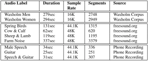
Audio Label Duration Sample Segments Source Rate

Waxholm Men 279sec 16K 2748 Waxholm Corpus Waxholm Women 294sec 16K 2949 Waxholm Corpus

Spring Birds 131sec 44.1K 1315 freesound.org Cow & Calf 62sec 48K 620 freesound.org Sheep & Lamb 119sec 48K 1195 freesound.org Farm Noise 337sec 48K 3379 freesound.org

Male Speech 34sec 44.1K 336 Phone Recording

Guitar 25sec 44.1K 251 Phone Recording

Speech & Guitar 31sec 44.1K 307 Phone Recording

Table 1: Specifications of audio datasets used in this study.

2.2.

Process

We kept preprocessing to an absolute minimum, in or-der to not make any assumptions at this stage. Each data set was used to produce a spectrogram (i.e. a visual representation of a fast Fourier transform) using the Sound EXchange Library6 (SOX), a standard library used to handle sounds. SOX seamlessly handles vary-ing frame rates and compression formats, which allowed us to avoid making decisions that may affect the data. The command line:sox soundfile -n spectrogram -l -r -m

-y Yresolution -X pixelpersec -o specfile generates 8-bit

greyscale spectrograms with a frequency range from 0 to 22000 Hz divided into 64 pixels along the Y-axis, and a temporal resolution of 1000 pixels per second along the X-axis. This format was used for all datasets.

The spectrogram and the corresponding audio recording were then split into equal-sized frames. For the purposes of this paper, a frame width of 100ms was used throughout, giving each spectrogram a height of 64 pixels, a width of 100 pixels, and a depth of 256 shades.

The spectrogram frames were used to distribute the sound snippets into hypothetically coherent regions in 2D space, where similar things are closer to each other and dissimilar things more apart. For this training we used a SOM im-plementation in TensorFlow(Abadi et al., 2015), in which the greyscale pixel values of the generated spectrograms are treated as input vectors to the algorithm.

The output is a set of 2D coordinates that are mapped to the audio segments. Each SOM was trained with 200 iter-ations over a grid. The size of the grid changed depending on the number of data points in each studied dataset, with a minimum of 30x30. Note that we do not attempt to do clustering on the output of the algorithm.

The resulting plot is amenable to sound browsing. In our implementation, the framework generates a visible grid (see Figure 1) where each datapoint is linked to its correspond-ing audio snippet. The correspondcorrespond-ing audio snippets are played when the cursor hovers over a given datapoint, so listeners can hover over different regions and listen to hy-pothetically similar data in quick succession or simultane-ously (Edlund et al., 2010)7_.

6

http://sox.sourceforge.net/ 7

The framework code is available for download8

For purposes of exploration, we used the interactive plots to point out regions where it was possible to make a clear judgment of (the majority) of the snippets, quickly and with little effort. These human judgments constitute the last step in our current process chain.

3.

Results

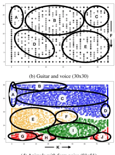
The panels in Figure 1 represent the results of our method, applied to four data sets. In each illustration, each data point (spectrogram) has been plotted as a circle with an opacity of 0.5, producing a darker effect where more than one data point is positioned in the same grid space. This visualises the SOMs. The areas marked with a black out-line represent areas where audio browsing of sounds close to each other in the SOM give a clear impression of the sound’s characteristics. Each such area is labeled, and the labels are used as references in the Discussion.

Figure 1a presents the visualisation of the studio recorded speech. There are no obvious clusters or regions discernible to the naked eye, except a darker area divided in two in the lower right corner (labeled G). Figure 1c show three clear regions that were coloured manually according to which recording session the point is associated with. Each ses-sions contains one animal type only, and is recorded on a separate occasion. The SOM training has resulted in three regions separated by empty grid cells (white regions) cor-responding well to the three sessions present in the data. In Figure 1d, we see five regions separated by strings of empty cells. Apart from the blue (triangle) region, that represents the added data, the other data is identical to that of the pre-vious figure. We see a separation of two regions of the red (cross) class, that is not present in the previous figure1c. Finally, in Figure 1b, we have a similar situation as in 1a: there are no obvious clusters. Instead, the data points seem evenly distributed over the grid.

The black outlines represent areas for which listeners re-ported that they could hear identifiable characteristics that separated the area from the surrounding areas with ease. The labels should read roughly as follows:

1a A: Vowels, resembles voice, can hear gender. high vol-ume; 1a B: transitions from fricatives to vowels; 1a C: frica-tives; 1a D: fricatives and quiet consonants; 1a E: short, truncated vowels; 1a F: sharp, non-human click; 1a G: si-lence/weak noises; 1a H: the arrow represents and overall increase in intensity.

1b A: Consonants. Sometimes alone, sometimes with gui-tar; 1b B: all voice; 1b C: very quiet, basically silence; 1b D: all guitar; 1b E: intensity generally increases top to bot-tom.

1c A: Very quiet, weak cow sounds; 1c B: calm soar of bird chirping; 1c C: loud cow sounds; 1c D: only sheep, loud at bottom and weaker sounds at top of region; 1c E: high-pitched, specific and loud bird chirping; 1c F: inten-sity generally increases top to bottom.

(a) Speech (76x76) (b) Guitar and voice (30x30)

(c) Animals (56x56) _{(d) Animals with farm noise (81x81)}

Figure 1:SOMs based on different sound recordings. The colour-coded informationwas not visible to, nor derived from the process, but added manually for purposes of illustration: (red=birds; green=sheep; yellow=cows, blue=farm sounds). The circled and labeled areas represent manual selections of perceptually clearly similar sounds, based on audio browsing.

left and louder to the right; 1d J: loud cow sounds; 1d K: intensity generally increases left to right.

4.

Discussion & future work

Although we have only taken first steps towards combin-ing dimensionality reduction and visualisation techniques with novel audio browsing techniques, our first results are quite promising. For the speech only data in 1a, a listener can quickly point out areas that are silent, that mainly con-tain vowels, and several other typical speech features. The next step here is to use the data in these relatively straight-forward areas to train models. The silence, for example, will let us model silence in the recording, which will make it possible to segment the data on silence - something that is not easily done in many recordings without spending an inordinate amount of time labeling silent segments sequen-tially and manually. The vowels may likewise be used to train a vowel model, and separate vowels from other sound of high intensity. We may also find oddities: the tapping noise in F turns out to be the press of a space bar, upon closer inspection of the original data. It turns out that the recorded individuals were told to tap the space bar between each utterance in this particular recording. For the gui-tar+voice data (1b), we quickly find vicinities with nothing but voice and nothing but guitar. Again, this information can be used to create models or to inform a second clus-tering, effectively creating a reinforcement learning setup. For animals (1c and 1d), we see that sounds that differ in a distinct manner indeed end up further apart. At this stage, we cannot tell whether it is the recording conditions or the animal noises, or both, that have the greatest influence, yet it is clear that the method we propose would work fairly

well to separate different (but unknown) datasets.

guitars some sequence contains. From this we get crude labels for each sound segment that can be used in a num-ber of applications, e.g. for search or as training data for supervised machine learning tasks.

5.

Acknowledgements

This work is funded in full by Riksbankens Jubileumsfond (SAF16-0917: 1). Its results will be made more widely accessible through the infrastructure supported by SWE-CLARIN (Swedish Research Council 2013-02003).

6.

Bibliographical References

Abadi, M., Agarwal, A., Barham, P., Brevdo, E., Chen, Z., Citro, C., Corrado, G. S., Davis, A., Dean, J., Devin, M., Ghemawat, S., Goodfellow, I., Harp, A., Irving, G., Is-ard, M., Jia, Y., Jozefowicz, R., Kaiser, L., Kudlur, M., Levenberg, J., Man´e, D., Monga, R., Moore, S., Mur-ray, D., Olah, C., Schuster, M., Shlens, J., Steiner, B., Sutskever, I., Talwar, K., Tucker, P., Vanhoucke, V., Va-sudevan, V., Vi´egas, F., Vinyals, O., Warden, P., Wat-tenberg, M., Wicke, M., Yu, Y., and Zheng, X. (2015). TensorFlow: Large-scale machine learning on heteroge-neous systems. Software available from tensorflow.org. Berg, J., Domeij, R., Edlund, J., Eriksson, G., House, D.,

Malisz, Z., Nylund Skog, S., and ¨Oqvist, J. (2016). Till-tal – making cultural heritage accessible for speech re-search. In CLARIN Annual Conference 2016, Aix-en-Provence, France.

Bertenstam, J., Mats, B., Carlson, R., Elenius, K., Granstr¨om, B., Gustafson, J., Hunnicutt, S., H¨ogberg, J., Lindell, R., Neovius, L., Nord, L., de Serpa-Leitao, A., and Str¨om, N. (1995). Spoken dialogue data collected in the Waxholm project.STL-QPSR, (49-74).

De Wet, F., Weber, K., Boves, L., Cranen, B., Bengio, S., and Bourlard, H. (2004). Evaluation of formant-like features on an automatic vowel classification task. The Journal of the Acoustical Society of America, 116(3):1781–1792.

Edlund, J. and Gustafson, J. (2016). Hidden resources -strategies to acquire and exploit potential spoken lan-guage resources in national archives. In Nicoletta Calzo-lari (Conference Chair), et al., editors,Proceedings of the Tenth International Conference on Language Resources and Evaluation (LREC 2016), Paris, France, may. Euro-pean Language Resources Association (ELRA).

Edlund, J., Gustafson, J., and Beskow, J. (2010). Cocktail– a demonstration of massively multi-component audio en-vironments for illustration and analysis. SLTC 2010, page 23.

Gregory, I. N. and Ell, P. S. (2007). Historical GIS: tech-nologies, methodologies, and scholarship, volume 39. Cambridge University Press.

Kohonen, T., Oja, E., Simula, O., Visa, A., and Kangas, J. (1996). Engineering applications of the self-organizing map. Proceedings of the IEEE, 84(10):1358–1384. Kohonen, T. (1982). Self-organized formation of

topo-logically correct feature maps. Biological Cybernetics, 43(1):59–69.

Pestian, J. P., Sorter, M., Connolly, B., Bretonnel Co-hen, K., McCullumsmith, C., Gee, J. T., Morency, L.-P.,

Scherer, S., and Rohlfs, L. (2017). A machine learn-ing approach to identifylearn-ing the thought markers of suici-dal subjects: a prospective multicenter trial.Suicide and life-threatening behavior, 47(1):112–121.

Sacha, D., Asano, Y., Rohrdantz, C., Hamborg, F., Keim, D., Brau, B., and Butt, M. (2015). Self organizing maps for the visual analysis of pitch contours. InProceedings of the 20th Nordic Conference of Computational Lin-guistics, NODALIDA 2015, May 11-13, 2015, Vilnius, Lithuania, number 109, pages 181–189. Link¨oping Uni-versity Electronic Press.

Sylwester, K. and Purver, M. (2015). Twitter language use reflects psychological differences between democrats and republicans. PloS one, 10(9):e0137422.

Thill, J.-C., Kretzschmar, W. A., Casas, I., and Yao, X. (2008). Detecting geographic associations in english di-alect features in north america within a visual data min-ing environment integratmin-ing self-organizmin-ing maps. Self-organising maps: applications in geographic informa-tion science, pages 87–106.

van der Maaten, L. and Hinton, G. E. (2008). Visualizing high-dimensional data using t-sne. Journal of Machine Learning Research, 9:2579–2605.