Lexical C o n c e p t A c q u i s i t i o n From C o l l o c a t i o n M a p 1
Young S. Han, Young Kyoon Han, and Key-Sun Choi
Computer Science Department
Korea Advanced Institute of Science and Technology Taejon, 305-701, Korea
[email protected], [email protected]
Abstract
This paper introduces an algorithm for automatically acquiring the conceptual struc- ture of each word from corpus. T h e concept of a word is defined within the proba- bilistic framework. A variation of Belief Net n a m e d as Collocation M a p is used to compute the probabilities. T h e Belief Net captures the conditional independences of words, which is obtained from the cooccurrence relations. T h e computation in general Belief Nets is k n o w n to be NP-hard, so w e adopted Gibbs sampling for the approximation of the probabilities.
T h e use of Belief Net to model the lexical meaning is unique in that the network is larger than expected in most other applications, and this changes the attitude toward the use of Belief Net. T h e lexical concept obtained from the Collocation M a p best reflects the subdomain of language usage. T h e potential application of conditional probabilities the Collocation Map provides may extend to cover very diverse areas of language processing such as sense disambiguation, thesaurus construction, automatic indexing, and document classification.
1
I n t r o d u c t i o n
T h e level o f the c o n c e p t u a l r e p r e s e n t a t i o n o f words can be very c o m p l e x in certain con- texts, b u t in t h i s p a p e r we a s s u m e r a t h e r s i m p l e s t r u c t u r e in which a concept is a set o f weighted a s s o c i a t e d words. We propose an a u t o m a t i c concept a c q u i s i t i o n f r a m e w o r k based on the c o n d i t i o n a l p r o b a b i l i t i e s s u p p l i e d d by a network r e p r e s e n t a t i o n o f lexical re- lations. T h e network is in the s p i r i t of Belief Net, b u t the p r o b a b i l i t i e s are not necessarily Bayesian. In fact this v a r i a t i o n o f Bayesian Net is discussed recently by (Neal, 1992). We e m p l o y e d t h e Belief Net with non Bayesian p r o b a b i l i t i e s as a base for r e p r e s e n t i n g t h e s t a t i s t i c a l r e l a t i o n s a m o n g concepts, a n d i m p l e m e n t e d the d e t a i l s o f the c o m p u t a t i o n .
the texts. The probabilities on dependent variables are computed from the frequencies, so the probability is now of objective nature rather than Bayesian.
The variation of Belief Net we use is identical to the sigmoid Belief Net by Neal (1992). In ordinary Belief Nets, 2 ~ probabilities for a parent variable with n children should be specified. This certainly is a burden in our context in which the net may contain even hundred thousands of variables with heavy interconnections. Sigmoid interpretation of the connections as in artificial neural networks provides a solution to the problem without damaging the power of the network. Computing a joint probability is also exponential in an arbitrary Belief network, thus Gibbs sampling which originates from Metropolis algorithm introduced in 50's can be used to approximate the probabilities. To speed up the convergence of the sampling we adopted simulated annealing algorithm with the sampling. The simulated annealing is also a descendant of metropolis algorithm, and has been frequently used to compute an optimal state vector of a system of variables.
From the Collocation Map we can compute an arbitrary conditional probabilities of variables. This is a very powerful utility applicable to every level of language processing. To name a few automatic indexing, document classification, thesaurus construction, and ambiguity resolution are promising areas. But one big problem with the model is that it cannot be used in real time applications because the Gibbs sampling still requires an ample amount of computation. Some applications such as automatic indexing and lexical concept acquisition are fortunately not real time bounded tasks. We are currently undertaking a large scale testing of the model involving one hundred thousand words, which includes the study on the cost of sampling versus the accuracy of probability.
To reduce the computational cost in time, the multiprocessor model that is success- fully implemented for Hopfield Network(Yoon, 1992) can be considered in the context of sampling. Other options to make the sampling efficient should be actively pursued, and their success is the key to the implementation of the model to the real time problems.
2
D e f i n i t i o n of Lexical C o n c e p t
Whenever we think of a word, we are immediately reminded of some form of meaning of the word. The reminded structure can be very diverse in size and the type of the information that the structure delivers. Though it is not very clear at this point what the structure is and how it is derived, we are sure that at least some type of the reminded structure is readily converted to the verbal representation. Then the content of vebral form must be a clue to the reminded structure. The reminded structure is commonly referred to as the meaning of a word. Still the verbal representation can be arbitrarily complex, yet the representation is made up of words. Thus the words in the clue to the meaning of a word seem to be an important element of the meaning.
Now define the concept of a word as
D e f i n i t i o n 1 The lexical concept of a word is a set of associated words that are weighted by their associativeness.
theories, but we believe it is more of inductive(experimental) process. Now define the concept a of word w as a probabilistic distribution of its associated words.
= { (w,, p d } , (l)
where
pi = P(Wl I w ) , a n d
p i > T .
Thus the set of associated words consists of those whose probability is above threshold value T. The probabilistic distribution of words may exist independently of the influence of relations among words though it is true that relations in fact can affect the distribution. But in this paper we do not take other information into the model. If we do so, the model will have the complexity and sophistication of knowledge representation. Such an approach is exemplified by the work of Goldman and Charniak (1992).
Equation 1 can be further elaborated in several ways. It seems that the concept of a word as in Equation 1 m a y not be sufficient. T h a t is, Equation 1 is about the direct association of a given word. Indirect association can also contribute to the meaning of a word. Now define the expanded concept of a word as
a ' ( w ) = { (wi, Pi)} U { (vi, qi)}, (2)
Ors
where
qi = P ( vi I o'(w)) ,and qi > T .
= { (w,, pl)} u (3)
If the indirect association is repeated for several depths a class of words in particular aspects can be obtained. A potential application of Equation 3 and 4 is the automatic thesaurus construction. Subsumption relation between words may be computed by care- fully expanding the meaning of the words. The subsumption relation, however, may not be based on the meaning of the words, but it rather be defined in statistical nature.
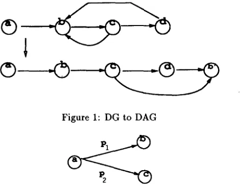
Figure 1: DG to DAG
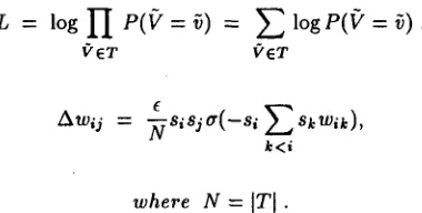
Figure 2: Word Dependency in Collocation Map
3
C o l l o c a t i o n Map
Collocation m a p is a kind of Belief Net or knowledge m a p t h a t represents the dependencies a m o n g words(concepts). As it does not have decision variables and utility, it is different from influence diagram. One problem with knowledge m a p is that it does not allow cycles while words can be m u t u a l l y dependent. Being DAG is a big advantage of the formalism in c o m p u t i n g probabilistic decisions, so we cannot help but stick to it. A cyclic relation should be broken into linear form as shown in figure 1. Considering the size of collocation m a p and the connectivity of nodes in our context is huge it is not practical to maintain all the combination of conditional probabilities for each node. For instance if a node has n conditioning nodes there will be 2 n units of probability information to be stored in the node. We limit the scope to the direct dependencies denoted by arcs.
W h a t follows is about the dependency between two words. In figure 2,
P ( b l a ) = pl,
(4)
P ( c l a ) = p2.
(5)
Pl denotes the probability t h a t word b occurs provided word a occurred. Once a text is transformed into an ordered set of words, the list should be decomposed into binary relations of words to be expressed in collocation map. Here in fact we are making an implicit assumption t h a t if a word physically occurs frequently around another word, the first word is likely to occur in the reminded structure of the second word. In other words, physical occurrence order m a y be a cause to the formation of associativeness a m o n g words.
Di = ( a , b , c , d , e , f , . . . , z ) .
[image:4.612.183.418.48.231.2]s
D i = (ab, ac, bc, ad, bd, cd, b e , c e , d e , c f , . . . , ) .
For words di and ct, P ( c tldi) can be computed at least in two ways. As mentioned earlier, we take the probability in the sense of frequency rather than belief. In the first method,
P(c~ldi) ~ f ( c t d i )
(6)
y(d~) '
where i < j.
Each node di in the m a p maintains two variables f(di) and f ( d i e j ) , while each arc keeps the information of P(cjldi). From the probabilities in arcs the joint distribution over all variables in the m a p can be computed, then any conditional probability can be computed. Let S denote the state vector of the map.
P ( g = ~) = H P ( S i = silS t = sj : j < i) . (7)
i
Computing exact conditional probability or marginal probability requires often exponen- tial resources as the problem is know to be NP-hard. Gibb's sampling must be one of the best solutions for computing conditional or marginal probabilities in a network such as collocation map. It approximates the probabilities, and when optimal solutions are asked simulated annealing can be incorporated. Not only for computing probabilities, pattern completion and pattern classification can be done through the m a p using Gibb's sampling. In Gibb's sampling, the system begins at an arbitrary state or a given S, and a free variable is selected arbitrarily or by a selecting function, then the value of the variable will be alternated. Once the selection is done, we m a y want to compute P ( S = g) or other fimction of S. As the step is repeated, the set of S's form a sample. In choosing the next variable, the following probability can be considered.
p ( s ~ = xlSt = s~ : j ¢ i) P ( S t = xlSt = st : j < i ) .
I ~ p ( s t = st ISi = ~, & = ,k : k < j, k ¢ i). (8) j>i
T h e probability is acquired from samples by recording frequencies, and can be up- dated as the frequencies change. The second method is inspired by the model of (Neal 1992) which shares much similarity with Boltzmann Machine. The difference is that the collocation m a p has directed ares. The probability that a node takes a particular value is measured by the energy difference caused by the value of the node.
P ( S i = silSj = sj : j < i) = o'(si E sjwij) . j<i
H i d d e n U n i t s
Figure 3: Collocation Map with Hidden Units
1
where a(t) -l + e - t A node takes -1 or 1 as its value.
P ( S = g ) = I I P ( S i = s i l S ¢ =s¢ : j < i ) i
= H a ( s ' E s j w ' i ) " (10) i i<i
Conditional and marginal probabilities can be approximated from Gibb's sampling. A selection of next node to change has the following probability distribution.
P(S~ = xIS j = sj : j # i)
+
(11)
j < i j > i k < j , k ~ i
The acquisition of probability for each arc in the second method is more complicated than the first one. In principle, the general patterns of variables cannot be captured without the assistance of hidden nodes. Since in our case the pattern classification is not an absolute requirement, we m a y omit the hidden nodes after careful testing. If we employ hidden units, the collocation m a p may look as in figure 5 for instance.
Learning is done by changing the weights in ares. As in (Neal, 1992), we adopt gradient ascent algorithm that maximize log-likelihood of patterns.
L = l o g H P(V =v) = E l ° g P ( V = O ) '
(12)
V'ET 17' E T
E
ZXwij = ~ s l s j o ' ( - s l ~ SkWik), (13)
k<i
where N = ]T[ .
[image:6.612.185.375.469.565.2]that whole learning is readjusted every time a new document is to be learned. Gradual learning(non batch) m a y degrade the performance of pattern classification probably by a significant degree, but what we want to do with collocation m a p is not a clear cut pattern identification up to each learning instance, but is a much more brute categorization. One way to implement the learning is first to clamp the nodes corresponding to the input set of binary dependencies, then run Gibb's sampling for a while. Then, add the average of energy changes of each arc to the existing values.
So far we have discussed about computing the conditional probability from Collocation Map. But the use of the algorithm is not limited to the acquisition of lexical concept. The areas of the application of the Collocation Map seems to reach virtually every corner of natural language processing and other text processing such as automatic indexing. An indexing problem is to order the words appearing in a document by their relative importance with respect to the document. Then the weight ¢(wi) of each word is the probability of the word conditioned by the rest of the words.
ek(wi) = P( wi l wj, j 5k i) . (14) The application of the Collocation Map in the automatic indexing is covered in detail in Han (1993).
In the following we illustrate the function of Collocation Map by way of an example. The Collocation Map is built from the first 12500 nouns in the textbook collection in Penn Tree Bank. Weights are estimated using the mutual information measure. The topics of the textbook used includes the subjects on planting where measuring by weight and length is frequently mentioned. Consider the two probabilities as a result of the sampling on the Collocation Map.
P(depthlinch ) = 0.51325, and
P(weightlinch ) = 0.19969.
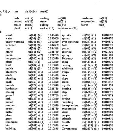
When the sampling was loosened, the values were 0.3075 and 0 respectively. The first version took about two minutes, and the second one about a minute in Sun 4 workstation. The quality of sampling can be controlled b y adjusting the constant factor, the cooling speed of temperature in simulated annealing, and the sampling density. The simple ex- periment agrees with our intuition, and this demonstrates the potentail of Collocation Map. It, however, should be noted that the coded information in the Map is at best local. When the Map is applied to other areas, the values will not be very meaningful. This may sound like a limitation of Collocation Map like approach, but can be an advantage. No system in practice will be completely general, nor is it desirable in m a n y cases. Figure 4 shows a dumped content of node tree in the Collocation Map, which is one of 4888 nodes in the Map.
4
C o n c l u s i o n
< h23 >
f:
b:
tree
di(36494) ctr(92)
inch
mi(19)
rooting
mi(20)
resistance
mi(21)
period mi(22)
straw
mi(31)
evaporation mi(32)
mulch mi(29)
pulling
mi(34)
flower
mi(5)
plant
mi(1)
root mi(13) moisture mi(28)
shrub
mi(24) c ( 4 )
0.043478
water
mi(26) c ( 3 )
0.032609
under-watering mi(36) c ( 1 )
0.010870
fertilizer
mi(59) c ( 3 )
0.032609
tree
mi(58) c ( 5 )
0.054348
March
mi(54) c ( 2 )
0.021739
pecan
mi(102) c(2) 0.021739
temperature
mi(106) c(1) 0.010870
plant
mi(9) c ( 1 )
0.010870
fruit
mi(107) c(1) 0.010870
mulch
mi(33) c ( 1 )
0.010870
blueberry
mi(123) c(1)
0.010870
shade
mi(130) c(4)
0.043478
planting
mi(155) c(1) 0.010870
bank
mi(350) c(1) 0.010870
branch
mi(172) c(1)
0.010870
landscape
mi(368) c(2)
0.021739
cooling
mi(586) c(1) 0.010870
ground
mi(126) c(2) 0.021739
inch
mi(133) c(1)
0.010870
period
mi(181) c(1) 0.010870
position
mi(596) c(1) 0.010870
mi(605) c(2)
0.021739
metal
mi(612) c(1) 0.010870
place
mi(443) c(1) 0.010870
grass
mi(381) c(1)
0.010870
command
mi(1815)
c(1) 0.010870
bird
mi(701) c(1) 0.010870
building
mi(307) c(1) 0.010870
sprinkler
mi(25) c ( 1 )
0.010870
system
mi(35) c ( 1 )
0.010870
over-watering mi(37) c ( 1 )
0.010870
hole
mi(60) c ( 1 )
0.010870
pound
mi(61) c ( 3 )
0.032609
growing
mi(105) c(2)
0.021739
spring
mi(42) c ( 2 )
0.021739
February
mi(38) c ( 2 )
0.021739
thing
mi(43) c ( 1 )
0.010870
cutting
mi(114) c(1)
0.010870
rabbiteye
mi(122) c(1)
0.010870
ajuga
mi(124) c(1) 0.010870
area
mi(131) c(1)
0.010870
slope
mi(132) c(1)
0.010870
trunk
mi(225) c(5)
0.054348
myrtle
mi(194) c(2)
0.021739
heating
mi(585) c(1)
0.010870
step
mi(588) c(1)
0.010870
root
mi(141) c(4)
0.043478
drying
mi(590) c(1) 0.010870
crowding
mi(595) c(1)
0.010870
transplanting
mi(594) c(1)
0.010870
evaporation
mi(609) c(1) 0.010870
stake
mi(613) c(3)
0.032609
people
mi(267) c(1)
0.010870
triangle
mi(616) c(1) 0.010870
breath
mi(1334) c(1) 0.010870
stone
mi(1813) c(1) 0.010870
Government
mi(2337) c(1) 0.010870
[image:8.612.112.502.56.501.2]of lexical concept. The representation named Collocation Map is a variation of Belief Net that uses sigmoid function in summing the conditioning evidences. The dependency is not as strong as that of ordinary Belief Net, but is of event occurrence.
The potential power of Collocation Map can be fully appreciated when the computa- tional overhead is further reduced. Several options to alleviate the computational burden are also begin studied in two approaches. The one is parallel algorithm for Gibbs sampling and the other is to localize or optimize the sampling itself. Preliminary test on the Map built from 100 texts shows a promising outlook, and we currently having a large scale testing on 75,000 Korean text units(two million word corpus) and Pentree Bank. The aims of the test include the accuracy of modified sampling, sampling cost versus accuracy, comparison with the Boltzman machine implementation of the Collocation Map, Lexical Concept Acquisition, thesaurus construction, and sense disambiguation problems such as in PP attachment and homonym resolution.
R e f e r e n c e s
[1] Baker, J. K. 1979. Trainable grammars for speech recognition. Proceedings of Spring Conference of the Acoustical Society of America, 547-550. Boston, MA.
[2] Ackley, G.E. Hinton and T.J. Sejnowski. (1985). A Learning Algorithm for Boltzmann machines, Cognitive Science. 9. 147-169.
[3] Cho, Sehyeong, Maida, Anthony S. (1992). "Using a Bayesian Framework to Identify the Referents of Definite Descriptions." AAAI Fall Symposium, Cambridge, Mas- sachusetts.
[4] Dempster, A.P. Laird, N.M. and Rubin, D.B. (1977). Maximum likelihood from in- complete data via the EM algorithm, J. Roy. Star. Soc. B 39, 1-38.
[5] Gelfan, A.E. and Smith, A.F.M. (1990). Sampling-based approaches to calculating marginal densities, J. Am. Star. Assoc 85. 398-409.
[6] Goldman, Robert P. and Charniak Eugene. (1992). Probabilistic Text Understanding. Statistics and Computing. 2:105-114.
[7] aan,
Young S. Choi, Key-Sun. (1993). Indexing Based on Formal Relevancy ofBayesian Document Semantics. Korea/Japan Joint Conferenceon on Expert Systems, Seoul, Korea.
[8] Lauritzen and Spiegelhalter, D.J. (1988). Local computation with probabilities on graphical structures and their application to expert systems. J. Roy. Star. Soc. 50. 157-224.
[9] Metropolis, N. Rosenbluth, A. W. Teller, A.H. Teller and Teller, E. (1953). Equation of state calculations by fast computing machines. J. Chem. Phys. 21. 1087-1092. [10] Neal, R.M. (1992). Connectionist learning of belief network. Artificial Intelligence 56.
71-113.
[12] Schutze, Hinrich. (1992). Context Space, AAAI Fall Symposium Series, Cambridge, Massachusetts.
[13] Spiegelhalter D.. and Lauritzen, S.L.. (1990). sequential updating of conditional probabilities on directed graphical structures. Networks 20. 579-605.