Analysis of Tomita’s Algorithm for General Context Free Parsing

ANALYSIS OF T O M I T A ' S A L G O R I T H M FOR GENERAL C ON T E X T - F R E E PARSING1

JAMES R. KIPPS ([email protected])

The RA N D Corporation, Santa Monica, CA 90406

Abstract. A variation on Tom ita’s algorithm is analyzed in regards to its time and space complexity. It is shown to have a general time bound of 0 ( n p’+1), where n is the length of the input string and p

is the length of the longest production. A modified algorithm is presented in which the time bound is reduced to 0 ( n 3). The space complexity of Tom ita’s algorithm is shown to be proportional to n2 in the worst case and is changed by at most a constant factor with the modification. Empirical results are used to illustrate the trade off between time and space on a simple example. A discussion of two subclasses of context-free grammars th at can be recognized in 0 ( n2) and O(n) is also included.

1. I N T R O D U C T I O N

Algorithms for general context-free (CF) parsing, e.g., Earley’s algorithm (Earley, 1968) and the Cocke-Younger-Kasami algorithm (Younger, 1967), are necessarily less efficient than algorithms for restricted CF parsing, e.g., the LL, operator precedence, and LR algorithms (Aho and Ullman, 1972), because they must simulate a m ulti-path, nondeterministic pass over their inputs using some form of search, typically, goal-driven. While many of the general algorithms can be shown to theoretically perform as well as the restricted algorithms on a large subclass of CF grammars, due to the inefficiency of goal expansion the general algorithms have not been widely used as practical parsers for programming languages.

A basic characteristic shared by many of the best known general algorithms is th at they are top- down parsers. Recently, Tom ita (1985) introduced an algorithm for general CF parsing defined as a variation on standard LR parsing, i.e., a table-driven, bottom -up parsing algorithm. The benefit of this approach, is th at it eliminates the need to expand alternatives of a nonterminal at parse time (what Earley refers to as the predictor operation). For Earley’s algorithm, the predictor operation is one of two 0 ( n 2) components. While eliminating this operation would not change the algorithm ’s time bound of 0 ( n 3), it could be significant to practical parsing. It is of interest to analyze the complexity of T o m ita’s algorithm and see how it compares.

Upon examination, T om ita’s algorithm is found to have a general time complexity of 0 (n ^ +1), where n is as before and p is the length of the longest production in the source grammar. Thus, this algorithm achieves 0 ( n 3) for grammars in Chomsky normal form (Chomsky, 1959) but has potential for being worse when productions are of unrestricted lengths. In this paper, I present a modification of T om ita’s algorithm th at allows it to run in time proportional to n3 for gram m ars with productions of arbitrary lengths.

2. TOMITA'S ALGORITHM

The following is an informal description of Tom ita’s algorithm as a recognizer; familiarity with standard LR parsing is assumed. Tom ita views his algorithm as a variation on standard LR parsing. The algorithm takes a shift-reduce approach, using an extended LR parse table to guide its actions. The extended parse table records shift/reduce and reduce/reduce conflicts as multiple action entries, so the parse table can no longer be used for strictly deterministic parsing. The algorithm simulates a nondeterministic parse with pseudo-parallelism. It scans an input string xi • • xn from left to right, following all paths in a breath-first manner and merging like subpaths when possible to avoid redundant computations.

1 T h is work w as su p p o rte d by the D efense A dvan ced R esearch P r o je c ts A gency, under co n tract num ber M D A -903-85-C -0030.

The algorithm operates by maintaining a number of parsing processes in parallel. Each process

has a stack, scans the input string from left-to-right, and behaves basically the same as the single parsing process in standard LR parsing. Each stack element is labeled with a parse state and points to its parent, i.e., the previous element on a process’s stack. The top-of-stack is the current state of a process.

Each process does not actually m aintain its own separate stack. Rather, these “multiple” stacks are represented using a single directed acyclic (but reentrant) graph called a graph-structured stack.

Each stack element corresponds to a vertex of the graph. Each leaf of the graph acts as a distinct top-of-stack to a process. The root of the graph acts as a common bottom-of-stack. The edge between a vertex and its parent is directed toward the parent. Because of the reentrant nature of the graph (as explained below), a vertex may have more than one parent.

The leaves of the graph grow in stages. Each stage Ui corresponds to the zth symbol x, from the input string. After x, is scanned, the leaves in stage Ui are in a one-to-one correspondence with the algorithm ’s active processes, where each process references a distinct leaf of the graph and treats that leaf as its current state. Upon scanning x,+ i, an active process can either (1) add an additional leaf to

Ui, or (2) add a leaf to £/,•+1. Only processes th at have added leaves to f/j+i will be active when x*+2 is scanned.

In general, a process behaves in the following manner. On x<, each active process (corresponding to the leaves in U i-1) executes the entries in the action table for x< given its current state. When a process encounters multiple actions, it splits into several processes (one for each action), each sharing a common top-of-stack. When a process encounters an error entry, the process is discarded (i.e., its top-of-stack vertex sprouts no leaves into Ui by way of th at process). All processes are synchronized, scanning the same symbol at the same time. After a process shifts on Xj into Ui, it waits until there are no other processes th at can act on x, before scanning x,+ i.

The Shift Action. A process (with top-of-stack vertex v) shifts on Xi from its current state s to some successor state s' by

(1) creating a new leaf v' in Ui labeled s';

(2) placing an edge from v' to its top-of-stack v (directed towards v); and

(3) making v' its new top-of-stack vertex (in this way changing its current state).

Any successive process shifting to the same state s' in Ui is merged with the existing process to form a single process whose top-of-stack vertex has multiple parents, i.e., by placing an additional edge from the top-of-stack vertex of the existing process in Ui to the top-of-stack vertex of the shifting process. The merge is done because, individually, these processes would behave in exactly the same manner until a reduce action removed the vertices labeled s' from their stacks. Thus, merging avoids redundant com putation. Merging also ensures th at each lead" in any Ui will be labeled with a distinct parse state, which puts a finite upper-bound on the possible number of active processes and, thus, limits the size of the graph-structured stack.

The Reduce Action. A process executes a reduce action on a production p by following the chain of parent links down from its top-of-stack vertex v to the ancestor vertex from which the process began scanning for p earlier, essentially “popping” intervening vertices off its stack. Since merging means a vertex can have multiple parents, the reduce operation can lead back to multiple ancestors. When this happens, the process is again split into separate processes (one for each ancestor). The ancestors will correspond to the set of vertices at a distance v from v, where p equals the number of symbols in the right-hand side of the pth production. Once r luced to an ancestor, a process shifts to the state s'

indicated in the goto table for Dp (the nonterminal on the left-hand side of the pth production) given the ancestor’s state. A process shifts on a nonterminal much as it does a term inal, with the exception th at the new leaf is added to Ui_i rather than Ui] a process can only enter Ui by shifting on x,.

The algorithm begins with a single initial process whose top-of-stack vertex is the root of the graph-structured stack. It then follows the general procedure outlined above for each symbol in the input string, continuing until there are either no leaves added to Ux (i.e., no more active processes), which denotes rejection, or a process executes the accept action on scanning the n + 1st input symbol ‘H,’ which denotes acceptance.

3. ANALYSIS OF T O M I T A ’S A L G O R I T H M

In this section, a formal definition of Tom ita’s algorithm is presented as a recognizer for input string xi • • • xn . This definition is understood to be with respect to an extended LR parse table (with start state So) constructed from a source grammar G.

Notation. The productions of G are numbered arbitrarily 1, • • •, d, where each production is of the form Dp — Cpi • • Cpp (1 < p < d) and where p is the number of symbols on the right-hand side of the pth production.

Definition. The entries of the extended LR parse table are accessed with the functions ACTIONS and GOTO.

• ACTIONS(s,x) returns a set of actions from the action table along the row of state s under the column labeled x. This set will contain no more than one of a shift action shs' (shift to state s) or an accept action acc; it may contain any number of reduce actions re p (reduce using production p). An empty action set corresponds to an error.

• GOTO(s,£>p) returns a state s' from the goto table along the row of state s under the column labeled with nonterminal Dp .

Definition. Each vertex of the graph-structured stack is a triple (i, s, l), where i is an integer corresponding to the ith input symbol scanned (at which point the vertex was created as a leaf), 5 is a parse state (corresponding to a row of the parse table), and / is a set of parent vertices. The processes

described in the last section are represented implicitly by the vertices in successive £/,-’s. The root of the graph-structured stack, and hence the initial process, is the vertex (O,So,0).

The Recognizer. The recognizer is a function of one argument REC(x! • • • x„). It calls upon

the functions SHIFT(t;,.s) and REDUCE(u,p). SHIFT(v,s) either adds a new leaf to {/,• labeled

with parse state s whose parent is vertex v or merges vertex v with the parents of an existing leaf. REDUCE(u,p) executes a reduce action from vertex v using production p. REDUCE calls upon the function ANCESTORS(u,p), which returns the set of all ancestor vertices a distance of p from vertex v.

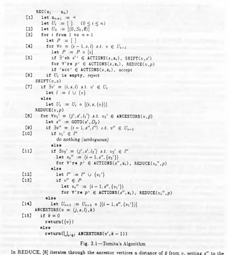
These functions, which vary somewhat from the formal definition given in Tom ita (1985),2 are defined in Figure 3.1.

In REC, [1] adds the end-of-9entence symbol H ’ to the end of the input string; [2] initializes the root of the graph-structured stack; [3] iterates through the symbols of the input string. On each symbol X,-, [4] processes the vertices (denoting the active processes) of successive C/,-_i’s, adding each vertex to

P to signify that it has been processed. On each vertex v, [5] executes the shift, reduce, and accept actions from the action table according to v's state s. After processing the vertices in {/<—ii [6] checks whether a vertex was added to ensuring th at at least one process is still active before scanning x,-+i.

In SHIFT, [7] shifts a process into state s by adding a vertex to £/, labeled s. If a vertex labeled s already exists, v is added to its parents, merging processes; otherwise, a new vertex is created with a single parent v.

2 T om ita’s functions REDUCE and REDUCE-E have been collapsed into a single REDUCE function; also

added were the A NC E ST O R S function and the concept of a “clone” vertex. W hile these changes do not alter T om ita’s algorithm significantly, they were helpful in developing ideas about its complexity.

REC(xi ••• xn )

[1] let xn+1 := H

let Ui := [ ] (0 < i < n)

[2] let U0 : = [(O, 5o ,0)j

[3] for i from 1 to n+ 1

let P := [ ]

[4] for Vv = (i — 1,5,/) 5./. u E U i - i

let P := P o [v]

[5] if 3 ‘ sh s'* € ACTIONS (s, x,) , SHIFT(v,s')

for V're p» € ACTI0NS(s,x.) , REDUCE(u.p)

if *acc’ € ACTIONS(s,Xj), accept

[6] if Ui is empty, reject

SHIFT( v , s )

[7] if 3vf = (i,s,l) s.t. v' £ Ui

let / := / U {u}

else

let Ui := Ui o [(i, s, {i/})] REDUCE(u,p)

[8] for Vt>i' = ( j ' ^ s ' J i ) s.t. vi' € ANCESTORS(v,p) let s" := GOTO ( s ' , Dp )

[9] if 3v" = { i - l , s " , l " ) s.t. v" 6 Ui_!

[10] if Vi' e I"

do nothing (am biguous) else

[11] if 3i?2; = {j ' y S' J ^) s.t. V2 € I" let vc" := (* - 1, s", {vi'})

for V're p* € ACTI0NS(5/',x.), REDUCE(yc",p) else

[12] let I" := I" U {u!7}

[13] if u" 6 P

let v," := (i- l,s", {iV})

for V're p» € ACTIONS(s^.x*), REDUCE( ,p)

else

[14] let := C/i-i o [(< - 1, s " , { v , 1})]

ANCESTORS (v = (j , s , l ) , k)

[15] if = 0

re tum({u})

else

r e t u m ( ( J v<€/ ANCESTORS(u'.jb - 1))

Fig. 3.1—T om ita’s Algorithm

In REDUCE, [8] iterates through the ancestor vertices a distance of p from v, setting s" to the state indicated in the goto table under Dv given the ancestor’s state s '. Each ancestor vertex v\ is shifted into U i-i on s " . [9] checks whether such a vertex v" already exists. (If not, [14] adds a vertex labeled s" to [/,•_i.) If v" does already exist, [10] checks th at a shift from the current ancestor vx' has not already been made. (If it has, then some segment of the input string has been recognized as an instance of the same nonterm inal Dp in two different ways, and the current derivation can be discarded as ambiguous; otherwise, vi' is merged with the parents of the existing vertex.) Before merging, [11] checks whether v\ is a “clone” vertex, created by [13] in an earlier call to REDUCE (as described below). If ui' is not a clone, [12] adds it to the parents of v " , merging processes. [13] checks if v"

has already been processed. If so, then it missed any reductions through rV. To correct this, v" is “cloned” into vc" (i.e., a variant on v" with a single parent u^), and all reduce actions executed on v"

are now executed on vc" .

Returning to [11], when reducing on a null production, ANCESTORS will return a clone vertex as the ancestor of itself. If a variant v-i of already exists in the parents of v " , then V\ is a clone of u2' . At this point v" has already been processed, meaning that there could still be reductions that have not gone through the single parent of ui'. To correct this, v" is again cloned, and all reduce actions executed on v" are executed on the new clone vc" .

Finally, in ANCESTORS, [15] recursively descends the chain of parents of vertex v, returning the set of vertices a distance of k from v.

The General Case. Tom ita’s algorithm is an 0 ( n /’+ l) recognizer in general, where p is the greatest p in G. The reasons for this are as follows:

(a) Since each vertex in Ui must be labeled with a distinct parse state, the number of vertices in any Ui is bounded by the number of parse states;

(b) The number of parents / of a vertex v — (i , s , l ) in Ui is proportional to i. Because processes could have begun scanning for some production p in each Uj (j < i), a process in Uicould reduce using p and split into ~ i processes (one for each ancestor in a distinct U j ) . Then each process could shift on Dp to the same state in Ui and, thus, that vertex could have ~ i

parents;

(c) For each x. + i, SHIFT will be called a bounded number of times (at most once for each vertex in Ui ) . SHIFT executes in a bounded number of steps.

(d) For each x,+i and production p, REDUCE(u,p) will be called a bounded number of times in REC, and REDUCE(uc",p) (the recursive call to REDUCE) will be called no more than — i

times. The reason for the former is the same as in (c). The latter is due to the conditions on the recursive call, which m aintain th at it can be called no more than once for each parent of a vertex in Ui, of which there are at most proportional to z;

(e) REDUCE(v,p), because at most ~ i vertices can be returned by ANCESTORS, executes in ~ i steps plus the steps needed to execute ANCESTORS.

(f) ANCESTORS(u,p) executes in ~ if steps in the worst case. While at most — i processes could have begun scanning for p, the number of paths by which any single process could reach v in Ui is bounded by the number of ways the intervening input symbols can be partitioned among the p vocabulary symbols in the right-hand side of production p. For a process th at started from Uj (j < *), the number of paths to v in Ui in the recognition of p can be proportional to

o o o

E l • £

i-mi =ji =mj

Summing from ; = 0, • • •, i gives a closed form proportional to if . A N C E S T O R S ^ ",p ), where

vc" = (», «{v'}), executes in ~ if ~ l steps because there is th at many ways ~ i ancestor vertices could reach v' and only one way v' could reach vc"\

(g) The worst case time bound is dominated by the time spent in ANCESTORS, which can be added to the time spent in REDUCE. Since REDUCE(v,p), with a bound ~ ip , is called only a bounded number of times, and REDUCE(uc//,p), with a time bound of ~ i?_1, is called at most ~ i times, the worst case time to process any x, is ~ i?, for each : = 0, • • •, n + 1 and longest production p\

(h) Summing from i = 0, • • •, n + 1 gives REC a general time bound proportional to n^+1. As a result, this bound indicates th at T om ita’s algorithm only belongs to complexity class 0 ( n 3) when applied to gram m ars in Chomsky normal form (CNF)3 or some other equally truncated notation.

3 In C N F, productions can have one of two forms, A —*■ BC or A —* a; thus, the length of the longest

production is at most 2.

Although any CF grammar can be autom atically converted to CNF (Hopcraft and Ullman, 1979), ex­ tracting useful information from derivation trees produced by such grammars would be time consuming at best (if possible at all).

4. M O D I F Y I N G T O M I T A ’S A L G O R I T H M FOR N 3 T I M E

In this section, T om ita’s algorithm is made an 0 { n 3) recognizer for CF grammars with productions of arbitrary length. Essentially, the modifications are to the ANCESTORS function. ANCESTORS is the only function th at forces us to use steps. It is interesting to note th at ANCESTORS can take this many steps even though it returns at most ~ i ancestor vertices and even though there are at most ~ i intervening vertices and edges between a vertex in U,- and its ancestors. This indicates that ANCESTORS can recurse down the same subpaths more than once. The efficiency of ANCESTORS and T om ita’s algorithm can be improved by eliminating this redundancy.

The modification described here turns ANCESTORS into a table look-up function. Assume there is a two-dimensional “ancestors” table. One dimension is indexed on the vertices in the graph- structured stack, and the other is indexed on integers k = 1, • • •, p, where p equals the greatest p. Each entry ( v, k) is the set of ancestor vertices a distance of k from vertex v. Then, ANCESTORS(v,fc) re­ turns the (at most) ~ i ancestor at (v, k) in — 1 steps. Of course, the table must be filled dynamically during the recognition process, so the time expended in this task must also be determined.

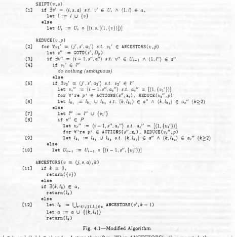
In Figure 4.1, ANCESTORS is defined as a table look-up function th at dynamically generates table entries the first time they are requested. In this definition, the ancestor table is represented by changing the parent field I of a vertex v = (i,s ,/) from a set of parent vertices to an ancestor field a. For a vertex v — (:, s, a), a consists of a set of tuples (k, /*), such th at It is the set of ancestor vertices a distance of k from v.

Figure 4.1 illustrates the necessary modifications made to the definitions of Figure 3.1; the function REC is unchanged. In SHIFT, [1] adds a vertex to Ui labeled s. If such a vertex does not already exist, one is created whose ancestor field records th at v is the ancestor vertex at a distance of 1; otherwise,

v is added to the other distance-1 ancestors.

In REDUCE, [2] iterates through the ancestor vertices a distance of p from v, setting s" to the state indicated in the goto table under Dp given the ancestor’s state s'. Each ancestor vertex v\ is shifted into Ui- 1 on s". [3] checks whether such a vertex v" already exists. (If not, [10] will add a vertex labeled s" to U i-1.) If v" does already exist, [4] checks that a shift from the current ancestor

v\ has not already been made. If it has, then vi' can be discarded as ambiguous; if not, then vi' can be merged with the other ancestors a distance of 1 from v " . Before merging, [5] checks whether ui' is a clone vertex as described in Section 3. If ui' is a clone (the result of being reduced on a null production), v" is again cloned, and all reduce actions executed on v" are executed on the new clone

vc" . After the application of REDUCE, [6] updates the ancestor table stored in v" to record entries made in the ancestor field a c" of the clone when k > 2. Otherwise, if vi' is not a clone, [7] adds it to the distance-1 ancestors of v", merging processes. [8] checks if v" has already been processed. If so, then it missed any reductions through v \ ', so v" is cloned into ve" and all reduce actions executed on

v" are now executed on v " . After reducing vc" , [9] updates the ancestor table stored in v" to record entries made in the ancestor field ac" of the clone when k > 2.

In ANCESTORS, [11] searches a (the portion of the ancestor table stored with v) for ancestor vertices at a distance of k from v. If an entry exists, those vertices are returned; if not, [12] calls ANCESTORS recursively to generated those vertices and, before returning the generated vertices, records them in the ancestor field of v.

The question now becomes how much time is spent filling the ancestor table. For

ANCESTORS(v,p), time is bounded in the worst case by ~ i2 steps, while for A N C ESTO R S^*",?), it is bounded by — i steps. In general, ANCESTORS(v,fc), where v = ( i,s ,a ) , will take ~ i steps to execute the first time it is called (one for each recursive call to ANCESTORS(t/,A: - 1), where

SHIFT(v.s)

[1] il 3v' = (z',s,a) s.t. v' G U{ A (1,/) 6 a,

let / := / U {v}

else

let U{ := C/i o [<i,s,[(l,{v})])]

REDUCE(v.p)

[2] for Vui' = ( j \ s ' , a x') s.t. v\' G ANCESTORS(u,p)

let s" := GOTO (s', D p )

[3] if 3v" = (z - 1, s", a") s.t. u" G tfi-i A ( l . H € a"

[4] if v\ G I"

do nothing (ambiguous) else

[5] if 3u2' = (j/,s/,a2/) s.t. u2' G I"

let we" := (z-l,s",ac") s.t. ac" = [(l>i'}>]

for V're p> G ACTIONS (s", x,) , REDUCE ( vc" ,p)

[6] let /fcl := /fcl U /fc3 s.t. € a" A (Ar, /*a) € ac" ( k >2)

else

[7] let I" := /" U { V }

[8] if v" G P

let uc" := (z - 1, s", a " ) s.t. ac"= [(1, {vi;})] for V're p> G ACTIONS(s",x ,), REDUCE(vc" ,p)

[9] let lkl := lkl U /*, s.t. (k , lkl) G a" A ( M * a) G ac" (fc>2)

else

[10] let U i - i := «/i_i o [(*- 1,*", {«!'})]

ANCESTORS ( v = ( j , s , a ) , k )

[11] if k = 0,

return({u})

else

if 3( k , / k) G a,

retun x d i e)

else

[12] let It := Uv'6M(l,/l)€a ANCESTORS (v' ,k - 1)

let a := a U { { k , l k)} retum(/fc)

Fig. 4.1— Modified Algorithm

v' G l\ and (l,/i) G a) and — 1 steps thereafter. When ANCESTORS(v,p) is executed, there are ~ z such “virgin” vertices between v and its ancestors, and so this call can execute ~ z2 steps in the worst case. ANCESTORS(vc",p) is called only after the call to ANCESTORS(v,p) has been made, where

ve" is a clone of v. This means th at ~ z of the vertices between v' and the ancestor vertices have been processed, so the call to A N CESTO RS(t/,p — 1) could take at most proportional to z steps for each of a bounded number of intervening vertices.

Given this, the upper bound on the number of steps th at can be executed by the total calls on REDUCE for a given x, is proportional to z2. Summing from z = 0, • • •, n -I- 1 gives ~ n3 steps as the worst case upper bound on the execution time of the modified algorithm.

5. SPACE B O U ND S

The space complexity of T om ita’s algorithm as it appears in Section 3 is proportional to n2 in the worst case. This is because the space requirements of the algorithm are bounded by the requirements of the graph-structured stack. There are a bounded number of vertices in each U, of the graph-structured stack, and each vertex can have at most ~ z parents. Summing again from i = 0, • • •, n + 1 gives — n 2 as the worst case space requirement for the graph-structured stack.

W i t h t h e m o d i f i c a t i o n o f S e c t i o n 4. t h e s p a c e r e q u ir e m e n t s o f th e g r a p h - s t r u c t u r e d s t a c k are in c r e a s e d b y a t m o s t a c o n s t a n t f a c t o r o f n 2 . T h i s is b e c a u s e th e m o d i f i c a t i o n r e p la c e s th e ~ i p a r e n t s o f a v e r t e x in U,- w i t h a t m o s t ~ pi en tr i e s in th e a n c e s t o r s field. S o , for a v e r t e x v = ( : , s , a ) s.t. v

G U , , t h e a n c e s t o r s field a w ill b e a s u b s e t o f { ( c , / c) | l < c < p) w h e r e |/ c | ~ i. S u m m i n g fr o m i — 0 | . . . ) n + 1 g i v e s <— pn2 or ~ n2 s t ill as a w o r s t ca se u p p e r b o u n d o n s p a c e .

6. E M P I RI CA L RESULTS

T h e v a r i a t i o n o n T o m i t a ’s a l g o r i t h m p r e s e n t e d in S e c t i o n 3 a n d t h e m o d i f i e d a l g o r i t h m p r e s e n t e d

in S e c t i o n 4 h a v e b o t h b e e n i m p l e m e n t e d in C. T h e g r a p h s in figures 6.1 a n d 6 .2 s h o w e m p i r i c a l

r e s u l t s c o m p a r i n g t h e t i m e a n d s p a c e r e q u i r e m e n t s o f b o t h i m p l e m e n t a t i o n s . E a c h t i m e / s p a c e g r a p h

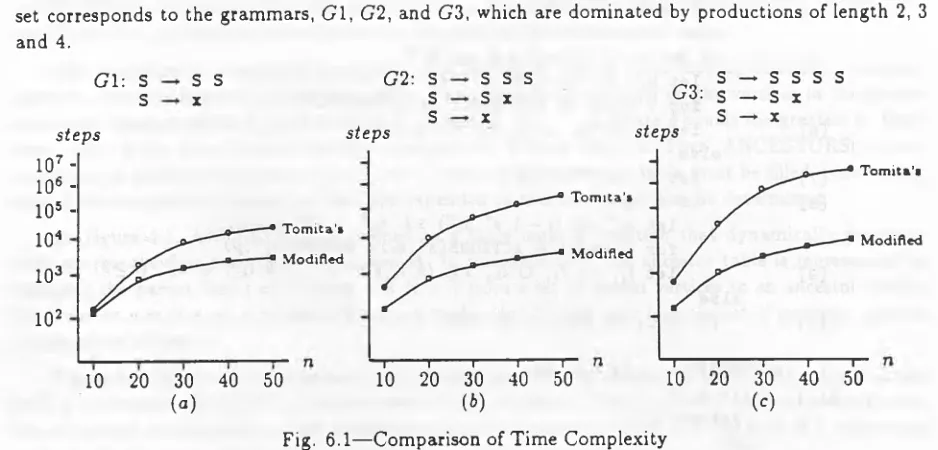
se t c o r r e s p o n d s t o t h e g r a m m a r s , G 1, G 2 , a n d G 3 , w h ic h are d o m i n a t e d by p r o d u c t i o n s o f l e n g t h 2, 3

a n d 4.

G1: S S

S S x

s t e p s

107 - 106 - 105 - 104

103

102

G2: S

S S s t e p s

S S S S x x

T o m i t a ’s

Modified

T o m i t a ’s

Modified

10 2 0 30 4 0 5o" (a)

1 i "i--- 1--- 1--- r~

10 20 30 4 0 50

(b)

Tom ita’s

M odified

“ i--- 1--- 1--- 1---r~

10 2 0 30 4 0 50

(c)

Fig. 6.1—Comparison of Time Complexity

The time graphs in Figure 6.1 measure the number of calls to SHIFT, REDUCE, and ANCES­ TORS. The input sentences are strings of x ’s of length 10 to 50. Our analysis of time complexity predicts th at the modified algorithm will take roughly the same number of steps for each grammar, while the steps taken by T om ita’s algorithm will increase as a function of the length of the dominant production. The empirical data gathered from our two implementations agrees with this prediction. When n = 50, the modified algorithm took ~ 7000 steps for gram m ar G1 in Figure 6.1 (a), ~ 6000 for G2 in Figure 6.1 (6), and — 10000 for G3 in Figure 6.1 (c); T om ita’s algorithm took ~ 44,000 steps for gram m ar G l, ~ 660, 000 for G2, and ~ 7, 300,000 for G3.

s p a c e s p a c e s p a c e

(a) (*) t o

Fig. 6.2—Comparison of Space Complexity

The space graphs in Figure 6.2 measure the number of edges required by the graph-structured stack (in T om ita’s algorithm ) and the length of entries in the ancestors table (in the modified algorithm). The number of vertices required is the same for both algorithms and is not counted; space th a t can be reclaimed before scanning successive x ,’s is also not counted. Our analysis of space complexity

predicts th at T om ita’s algorithm will require ~ n 2 space and that the modified algorithm will require at most a factor of n 2 additional space. The empirical evidence also agrees with this prediction. The space requirements of the modified algorithm differs from Tom ita’s algorithm by a factor of ~ 2.1 for gram m ar G1 in Figure 6.2 (a), ~ 3.9 for G2 in Figure 6.2 (6), and ~ 4.7 for G3 in Figure 6.2 (c).

7. LESS T H A N N 3 T I M E

Several of the better known general CF algorithms have been shown to run in less than 0 ( n 3) time for certain subclasses of grammars. Therefore, it is of interest to ask if Tom ita’s algorithm, as well as the modified version presented here, can also recognize some subclasses of CF grammars in less than 0 ( n 3) time. In this section, I informally describe two such subclasses that can be recognized in

0 ( n 2) and O(n) time, respectively. The arguments for their existence parallel those given by Earley (1968), where they are formally specified.

Time 0 (n2) Grammars. ANCESTORS is the only function that forces us to use ~ i? steps in Tom ita’s algorithm and ~ r steps in the modified algorithm. We determined th at this could happen when a ancestor vertex v' from Uj (j < i) reached the reducing vertex v in Ui by more than a single path, i.e., the symbols x;- • • • x, were derived from a nonterminal Dp in more than one way, indicating th at gram m ar G is ambiguous. If G were unambiguous, then there would be at most one path from a given v' to v. This means th at the bounded calls to ANCESTORS(t>,p) can take at most ~ steps and th at ANCESTORS(uc",p) can take at most a bounded number of steps. The first observation is due to the fact th at there are ~ i ancestor vertices that can be reached in only one way. Similarly, the second observation is due to the fact th at if A N C E S T O R S ^ ",p ) took ~ i steps, returning ~ i

ancestors, and was called ~ i times, then some ancestor vertices must have shifted into Ui in more than one way, which would be a contradiction, meaning gram m ar G must be ambiguous. So, if the gram m ar is unambiguous, then the total time spent in REDUCE for any x< is ~ i and the worst case time bound for the T om ita’s algorithm is 0 ( n 2). A similar result is true for the modified algorithm.

Tim e O(n) Grammars. In his thesis, Earley (1968) points out th at “ . . . for sc le grammars the number of states in a state set can grow indefinitely with the length of the string being recognized. For some others there is a fixed bound on the size of any state set. We call the latter grammars bounded state grammars.” While Earley’s “states” have a different meaning than states in Tom ita’s algorithm, a similar phenomena occurs, i.e., for the bounded state grammars there is a fixed bound on the number of parents any vertex can have. In T om ita’s algorithm, bounded state grammars can be recognized in time O (n) for the following reason. No vertex can have more than a bounded number of ancestors (if otherwise, then — i vertices could be added to the parents of some vertex in Ui, proving by contradiction th at the gram m ar is not bounded state). This means th at the ANCESTORS function can execute in a bounded number of steps. Likewise, REDUCE can only be called a bounded number of times. Summing over the x* gives us an upper bound ~ n. Again, a similar result is true for the modified algorithm. Interestingly enough, Earley states that almost all LR(k) grammars are bounded state, as well, which suggests that T om ita’s algorithm, given fc-symbol look ahead, should perform with little loss of efficiency as compared to a standard LR(fc) algorithm when the gram m ar is “close” to LR(fc). Earley also points out th at not all bounded state grammars are unambiguous; thus, there are non-LR(fc) gram m ars for which T om ita’s algorithm can perform with LR(&) efficiency.

8. C O N CL US I O N

The results in this paper support in part T om ita’s claim (1985) of efficiency for his algorithm. W ith the modification introduced here, T om ita’s algorithm is shown to be in the same complexity class as existing general CF algorithms. These results also give support to his claim th a t his algorithm should run with near LR(fc) efficiency for near LR(fc) grammars.

It should be noted th at while the modification to Tom ita’s algorithm has theoretic interest it would detract from a practical parser. Realistic grammars are constrained by the fact th at they must be hum an-readable. Since human-readable grammars should never realize the worst-case 0 (n ^ + l ) time

bound of T om ita’s algorithm, the benefits of the ancestors table in the modified algorithm would not balance out its overhead cost. In this regard, the modified algorithm should not be viewed as an “improvement” over T om ita’s algorithm but as a means of illustrating its place among other general CF algorithms.

The variation on Tom ita’s algorithm described in this paper, as well as the modified algorithm, have been implemented in both LISP a ..i C at The RAND Corporation. The LISP implementation (Kipps, 1988) is distributed with ROSIE (Kipps et al., 1987), a language for applications in artifi­ cial intelligence with a highly ambiguous English-like syntax. The C implementation is part of the RAND Translator-G enerator project, which is developing a “next generation” YACC4 for non-LR(fc) languages.

REFERENCES

Aho, A.V., J.D. Ullman, The Theory o f Parsing, Translation and Compiling, Prentice-Hall, Englewood Cliffs, NJ, 1972;

Chomsky, N., “On Certain Formal Properties of G ram m ars,” in Information and Control, vol. 2, no. 2, pp. 137-167, 1959.

Earley, J., An Efficient Context-Free Passing Algorithm, Ph.D. Thesis, Computer Science Dept.,

Carnegie-Mellon University, Pittsburg, PA, 1968.

Hopcraft, J.E ., J.D . Ullman, Introduction to A utom ata Theory, Languages, and Computation,

Addison-Wesley, Reading, MA, 1979.

Kipps, J.R ., B. Florman, H.A. Sowizral, The New RO SIE Reference Manual and User’s Guide, R- 3448-DARPA, The RAND Corporation, 1987.

Kipps, J.R ., “A Table-Driven Approach to Fast Context-Free Parsing,” N-2841-DARPA, The RAND Corporation, 1988.

Knuth, D.E., “On the Translation of Languages from Left to Right,” Information and Control, vol. 8, pp. 607-639, 1965.

Johnson, S.C., “YACC—Yet Another Compiler Compiler,” CSTR 32, Bell Laboratories, Murray Hill, NJ, 1975.

Tom ita, M., An Efficient Context-Free Parsing Algorithm for Natural Languages and Its Applications,

Ph.D. Thesis, Com puter Science Dept., Carnegie-Mellon University, Pittsburg, PA, 1985.

Younger, D.H., “Recognition and Parsing of Context-Free Languages in Time n3,” in Information and Control, vol. 10, no. 2, pp. 189-208, 1967.

4 YACC (Johnson, 1975) is a parser-generator for LALR(l) languages.