Entropy-Stabilized Oxides: Explorations of a Novel Class of Multicomponent Materials.

(1)

Abstract

ROST, CHRISTINA MARY. Entropy-Stabilized Oxides: Explorations of a Novel Class of Multicomponent Materials (Under the direction of Professor Jon-Paul Maria).

An ever-present challenge for scientists and engineers is to develop new materials that are innovative enough to set a new technological precedent and maintain application relevance for a substantial timeframe. There are many ways in which materials are exploited for new or improved properties, including but not limited to compositional substitution, doping, strain induction, or synthesis variation. The call for the Materials Genome Initiative has invoked the combined effort between theoreticians, experimentalists and industrialists to explore and apply material systems never before seen. One such strategy for new materials exploration is the development of high entropy alloys (HEAs). In HEAs, the addition of five or more component materials increases configurational entropy such that the resulting system contains fewer phases than traditionally expected, most of which are solid solutions. Research in this field is continuing to find new and exciting properties, with high potential for technological implementation.

(2)

(3)

(4)

Entropy-Stabilized Oxides: Explorations of a Novel Class of Multicomponent Materials

by

Christina Mary Rost

A dissertation submitted to the Graduate Faculty of North Carolina State University

in partial fulfillment of the requirements for the degree of

Doctor of Philosophy

Materials Science and Engineering

Raleigh, North Carolina

2016

APPROVED BY:

(5)

Dedication

(6)

Biography

Christina Mary Rost was born on February 15, 1987 to parents Allen and Cynthia Rost

of Speers Hill, Pennsylvania. After graduating Charleroi High School in 2005, Tina

enrolled as a double major in Physics and Physics Education with a minor in

mathematics at Indiana University of Pennsylvania. During her senior year of

undergraduate studies, Tina began research under Dr. Gregory Kenning working on the

relaxation time scales of magnetic spin-glasses. Upon graduation in 2009, Tina

remained working with Dr. Kenning in pursuit of a M.S. Physics degree where she

designed, built and automated a dual DC SQuID magnetometer for relaxation studies.

Meanwhile, she also held a graduate assistantship in the department of Liberal Studies,

docketing new course proposals for the University-Wide Undergraduate Curriculum

Committee. In 2011, she was hired as an adjunct faculty member within the IUP physics

department and taught undergraduate physics laboratory sequences to both major and

non-major classes. Tina joined the Complex Oxides and Thin Films Group at North

Carolina State University in 2012, under the direction of Dr. Jon-Paul Maria, in pursuit of

a Ph.D. in Materials Science and Engineering. Her work involved the development of a

new class of complex oxide systems, called Entropy-Stabilized Oxides. Since 2013,

(7)

Acknowledgements

Ultimately, I owe tremendous gratitude to my advisor, Dr. Jon-Paul Maria. If it weren’t

for his support, uncanny problem-solving abilities, and extreme optimism in the face of

impending scientific doom, I wouldn’t be writing this dissertation.

I wish to express my love and appreciation for my family. Glenn, my husband, whose

kindness and patience trumps any person I’ve ever known; my parents, Al and Cindy,

and my brother, A.J., who continue to support me unconditionally.

I cannot forget the past and present group members of the Complex Oxides and Thin

Films group: Dr. David Harris, Dr. Edward Sachet, Dr. Edward Mily, Chris Shelton, Alex

Smith, Xiaoyu Kang, Kyle Kelley, Luis Hernandez, and Richard Floyd. This also

includes visiting members: Gyung Hyung Ryu, Viktor Bauer, Trent Borman, and Scarlet

Kong. Never have I had the pleasure of working with such a great group of guys. Your

friendship and shared memories with stay with me forever.

I would also like to thank our collaborators; I’m lucky to be a part of such a great

(8)

List of Tables

Table 2.1 Table of EXAFS scattering cross sections, absorption lengths, and calculated

mass. ... 20

Table 3.1 Initial oxide components in alloy J14. *L denotes low spin, H denotes high spin. From R.D. Shannon and C.T. Prewitt, "Effective ionic radii in oxides and fluorides," Acta. Cryst., v. B25, p925, p. 5, 1969. ... 52

Table 3.2 List of compositions used to prepare the transition temperature phase diagrams in Figure 3.2(c-g) in the main text. ... 53

Table 3.3 Calculated relative intensity ratios for J14. ... 55

Table 3.4 Elements measured at APS beamline 12-BM-B. ... 55

Table 4.1 EXAFS cross sections, absorption coefficients, and absorption lengths for energy edged pertaining to Co, Ni, Cu and Zn cations. ... 66

Table 4.2 Results of best fits for Ni, Co, Zn and Cu cations in J14. ... 72

Table 5.2 List of components in each composition and their respective molar percentage: T22, J14C, and J30. ... 94

Table 5.3 Calculation of lattice parameter for T22 rocksalt gown on (100) Si. The calculated standard deviation is ± 0.004. ... 97

Table 6.1 List of compositions used in this study. ... 124

Table A.1 Compositions ... 175

(12)

List of Figures

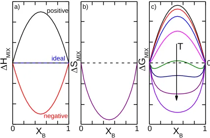
Figure 1.1 The typical materials development process. ... 1 Figure 1.2 Variation of thermodynamic mixing properties a) ∆Hmix, b) ∆Smix, and c) ∆Gmix

(13)

EDS maps show uniform spatial distributions for each element and are atomically resolved. ... 37 Figure 3.6 A binary metallic compared to a ternary oxide. A schematic representation of two lattices illustrating how the first near-neighbor environments between species having different electronegativity (the darker the more negative charge localized) for (a) a random binary metal alloy, and (b) a random pseudo-binary mixed oxide. In the latter, near-neighbor cations are interrupted by intermediate common anions. ... 41 Figure 3.7 Expanded view of one XRD temperature ladder showing the progression to single phase with 25 °C annealing steps. Red arrows indicate second phases, green and blue arrows indicate shoulders of second phases associated with wurtsitic and rocksalt structures respectively. Dashed lines highlight relative intensity values. Note that for rocksalt, I111 cannot be larger than I200, thus we can use the relative intensity

(14)

(15)

expanded in the J30 compared to the MgO (see panel [001]). J30 c/a measured to be 26.56 to 25.92 pixel; MgO c/a measured to be 25.85 to 25.86. ... 111 Figure 5.14 EDS map of J30 rocksalt showing the spatial distribution of constituent cations within one fcc sublattice, while oxygen occupies the other fcc sublattice. Observation of each map suggests an overall uniform cation distribution throughout the sampling area with minimal cation clustering. Mg appears to be brighter do to the fact that the system is detecting the MgO substrate in addition to the film. ... 111 Figure 5.15 Diffraction measurements taken of J30 grown on MgO at time t = 0, 4, 7, 15, and 425 days after growth. There appear to be no changes in the pattern suggesting a thermodynamically metastable film within the timescale of these measurements. ... 113 Figure 5.16 Examples of compositions that do not stabilize into a single phase form under bulk synthesis conditions up to 1650 °C. Composition J34 (MgxNixCoxCuxZnxSnxO, X = 0.1667) (top) depicts a series of phase transformations that

appear to approach a single phase rocksalt just above 1650 °C. At 1550 °C two primary phases are present: rocksalt and spinel. At 1650 °C only trace amounts of spinel remain. Composition J35 (MgxNixCoxCuxZnxCrxO, X = 0.1667) ... 115

Figure 5.17 Omega rocking curves of the (002) peak of the J30 film compared to the MgO substrate. The rocking curves were collected at the optimized 2θ positions for the film and substrate respectively. The substrate has a full-width-half-maximum (FWHM) value of 0.013 ° and the film has a FWHM of 0.018 °. ... 116 Figure 5.18 Original skew-symmetric measurement compilation for T22 grown on (100) Si. Comparison with Figure 5.4 shows the same phase present. Discrepancies between the images are a result of different optics used in the measurement. ... 117 Figure 6.1 Composition J30 (J14+Sc3+) grown on (100) MgO substrates at incremental deposition temperatures from 150 °C-700 °C. Crystalline growth begins near 300 °C and remains steady with the out-of-plane lattice parameter increasing linearly with temperature. Phase instability appears around 600 °C, and the system relaxes at 700 °C. ... 121 Figure 6.2 Plot of J30 lattice constant versus deposition temperature showing a linear increase in c(Å), with in-plane lattice constant remaining pinned to the substrate. 122 Figure 6.3 Diffraction patterns around the (200) substrate peak for ESO compositions containing a) Sb, b) Ge, c) Cr, and d) Sn. ... 126 Figure 6.4 Plot of compositions containing different sixth element additions Sn, Sb, Ge, Cr, and Sc. Each composition has a unique lattice constant trend. ... 127 Figure 6.5 J35 series grown on (0001) sapphire and (100) spinel substrates at incremental temperatures from 200 °C - 500 °C at 50 mTorr pO2. Phase separation occurs at 450 °C. The in-plane relationship of J35 grown on sapphire is shown in supplemental Figure 6.24. ... 129 Figure 6.6 Composition J35 grown on a) MgO, b) c-sapphire, and c) Spinel in 50 °C

(16)

350 °C, c remains constantly smaller than the substrate. At 400 °C and higher, c becomes larger than the substrate... 132 Figure 6.9 XRD diffraction pattern around the a) 200 MgO peak depicting complex interference which limits the accuracy of lattice parameter calculation b) the 204 skew-symmetric reflection enabling calculation of lattice parameter, c = 4.207Å. ... 133 Figure 6.10 J14 film grown on a polycrystalline alumina substrate resulting in a polycrystalline film with calculated lattice parameter consistent with the bulk value for cubic symmetry. ... 134 Figure 6.11 XRD scan of before and after post deposition anneal of J30 grown at 350 °C. ... 136 Figure 6.12 Diffraction series (a) of J35 grown at 10 mTorr pO2 from 250 °C–700 °C with corresponding lattice parameters and inferred instability regions (b). ... 139 Figure 6.13 Diffraction series (a) of J35 grown at 30 mTorr pO2 from 300 °C - 500 °C with corresponding lattice parameters and inferred instability regions (b). ... 140 Figure 6.14 Scatter plot of c versus deposition temperature for J35 grown on MgO under 10, 30 and 50 mTorr O2.Instability regions shift with temperature and O2

pressure, as evidenced by the appearance of (111) spinel peaks shown in supplementary Figure 6.23Diffraction patterns showing the temperature and pressure dependent development of a (111) spinel peak in composition J35 indicating phase separation into a rocksalt + spinel for a) 10mTorr O2, b) 30mTorr O2, and c) 50mTorr

O2.. ... 141

Figure 6.15Diffraction series of J35 grown at a) 300 °C in 10 – 50 mTorr O2 with b) the

corresponding exponential change in out-of-plane lattice constant versus O2. ... 142

Figure 6.16 Plot of c-lattice constant versus oxygen pressure for total pressure and partial pressure series. Regardless of the trend function, both systems experience a decrease in lattice parameter with increasing oxygen content. ... 144 Figure 6.17 Plots of c versus deposition temperature for a) the 10mTorr O2 series and

b) the 10mTorr O2 series. Again, while there is a slight shift in overall lattice parameter

between the pure O2 and the pO2 series, the overall trend of decreasing lattice constant

as temperature increases remain the same. ... 146 Figure 6.18 Plots of pre and post-annealed lattice parameters for a) J14 at 200 °C and 700 °C and b) J30 at 300 °C, 450 °C, and 700 °C. ... 147 Figure 6.19 XRD series depicting the change in out-of-plane lattice parameter for composition Mg1-xNixO with a) X = 0.01, b) X = 0.5, and c) X = 1.Films are

(17)

Figure 6.23Diffraction patterns showing the temperature and pressure dependent development of a (111) spinel peak in composition J35 indicating phase separation into

a rocksalt + spinel for a) 10mTorr O2, b) 30mTorr O2, and c) 50mTorr O2. ... 155

Figure 6.24 φ-scan of J35 grown on c-sapphire. The (104) sapphire planes exhibit three-fold symmetry along <0001>, while J35 exhibits three-fold symmetry along <111> with two directional domains oriented ± 30 ° to the substrate. ... 156

Figure B.1 Simplified schematic of a XAFS beamline. The most common (and perhaps most stable) measurement mode is transmission. If the samples do not meet the thickness criteria or contain a dilute species, a fluorescence detector may be a good alternative. Electron-yield is also a measurement mode for XAFS, but avoided entirely because it is never used in this work. ... 177

Figure B.2 The absorption and emission process. When x-rays are incident upon an elemental species with a core electron binding energy comparable with that of the light wave, a photoelectron is emitted in the form of a spherical wave. As the wave expands outward, it scatters from neighboring atoms. The interference between the forward and back scattering wave functions give rise to the EXAFS. ... 178

Figure B.3 Typical XAFS measurement before processing. The energy range spans 200eV below the known absorption edge of an element (pre-edge) to 800-1200eV above the edge depending on signal-to-noise ratio and whether there is another edge. The XANES region (not analyzed in this work) is approximately -30eV to 50eV around the absorption edge. Above 50eV is considered the EXAFS region. ... 180

Figure B.4 Raw data graphs of three consecutive XAFS measurements of the Ni absorber in J14. ... 183

Figure B.5 First derivative of a J14-Ni spectrum. The absorption edge should be marked as the first peak regardless of how intense it may be. ... 184

Figure B.6 First derivative of the Ni foil spectra. Again, the first peak is chosen to maintain consistency. The intensity of this peak versus the one of J14-Ni is due to the severity of the slope at the onset of the absorption edge. ... 185

Figure B.7 χ(k) spectrum showing glitches, denoted by arrows. ... 186

Figure B.8 Collective χ(k)spectra for all J14-Ni runs after glitch removal. ... 187

Figure B.9 Merged χ(k)spectrum containing all J14-Ni runs. Notice the signal to noise improvement over the individual scans. ... 188

Figure B.10 Pre and post-edge fitting for(E) normalization. ... 189

Figure B.11 Normalized (E). ... 190

Figure B.12 Background spline fit to (E) needed to isolate χ(k). ... 191

Figure B.13 Chosen range in χ(k) for Fourier transform and analysis. ... 192

Figure B.14 Resulting Fourier transform of the χ(k) spectrum. Most commonly used for model fitting. ... 193

(18)

Figure B.18 Fourier transform of χ(k) for J14 Ni, with a Hanning window between 1.05 and 3.35 Å, containing the individual scattering paths that are using during the fit.199 Figure B.19 Complete fit to the second nearest neighbor for J-14 Ni. ... 201 Figure B.20 Snapshot of fit report. σ2

(19)

1 Introduction

Materials and Technology

1.1

Materials development is the backbone of societal evolution and sustainability [1]–[3]. As a civilization continues to progress, technologies needed for advancement often become materials limited. Thus, it is the grand challenge of scientists and engineers to develop new systems that are innovative enough to set a new technological precedent and maintain application relevance. The standard methodologies in which materials are experimentally developed rely on modification of already well-understood systems to add or improve upon desired properties [4]. Figure 1.1 illustrates this process. The crystal chemistry work done by Pauling, Goldschmidt, and Hume-Rothery [5]–[7] predicted thermodynamically stable structures based on ionic radii of a given chemical constitution. Muller and Roy [8] compiled a significant review of such work, intended as a database for structure predictability, property relationships, and applications. It is on these works that the routes to materials development, both experimental and computational, are based.

Figure 1.1 The typical materials development process.

(20)

community uses substitution to increase charge capacity and improve cycling to find compositions suitable for alternatives to LiCoO2 [10]. Enhanced phase stability and

redox properties are found in thermoelectric systems, providing possible design guidelines for oxide converters [11]. The multifunctional materials [12] and multiferroics [13], [14] communities have benefitted from the use of chemical substitution as well.

Epitaxial strain has also proven to be an effective tool for modifying certain properties in a variety of thin film systems, which supersedes that of bulk or lattice-matched equivalents. Experimentalists who play the “strain game” [15] have found scientific improvements, such as enhanced carrier mobility and increased transconductance in high-electron-mobility transistors (HEMT)s [16] and metal-oxide-semiconductor field-effect transistors (MOSFET)s [17]. Inducing compressive strain in superconducting thin films finds that the critical temperature, TC, increases with an increasing out-of-plane

lattice constant [18], [19]. Similarly, the ferromagnetic Curie temperature can be tuned though varying tensile strain to the point of temperature saturation above a certain lattice constant [20]. Strain has even given rise to properties non-existent in bulk form, such as the induced room temperature ferroelectricity in SrTiO3 [21].

(21)

An Alternative Approach to Materials

1.2 Development

In 2004, Cantor et al. [31] took an alternative approach to conventional methods. They sought to explore the rather sparse, central regions of higher-order phase diagrams where compositions contain near equal amounts of components. In their original work, a 20-component and a 16-component metallic system containing equimolar amounts of elements from essentially every area of the periodic table were synthesized and characterized. Results show each system to be multiphase and brittle; however, a common single primary FCC phase existed -that was chemically rich in transition metals. Using this information, Cantor created six more compositions, each based on an equimolar standard: CrMnFeCoNi. They used this standard, and systematically added various sixth component metals including Cu, Ti, Nb, Ge and V. It was found that all synthesized alloys had a dendritic microstructure with a compositional preference, suggesting the solubility limitations of CrMnFeCoNi, between dendritic and inter-dendritic regions.

Cantor’s work inspired significant research efforts due to the fact that these materials seem to form significantly fewer phases than that dictated by the Gibbs Phase Rule [32], [33]. Yeh, et al. [34] attributed this phenomenon to high mixing entropy, ΔSmix

(= -R ∑ xi ln xi), and adopted the term “high entropy alloys” (HEAs). The maximum

(22)

associated with such a composition enhances mutual solubility among constituent species, resulting in minimum phase systems.

More recently [35], two definitions have been accepted as guidelines for the classification of this new family of alloys. The first of which is an extension of the 5 at.%-–35 at.% statement to include elements present in ≤ 5 at.% [36]. Constituents are classified into two categories, nXi defined as n ≥ 5 and 5 % ≤ xi ≤ 35%, and nXj defined

as n ≥ 0 and xj ≤ 5%. n corresponds to the number of components, and xm is the at.% of

the mth component in the composition. This definition yields three types of compositions: equimolar, non-equimolar, and minor elemental additions. The second definition is based solely on the entropy concept. Here, a HEA is defined as a composition that results in ΔSmix ≥ 1.5R where R is the gas constant, 8.314 J/mol∙K. Mixing entropies

above this value have a higher affinity for a solid solution [23].

In addition to the stated definitions, the community has agreed upon four core characteristics of HEAs that are expected to affect structure-property relationships (either directly or indirectly). For more rigorous details on the core characteristics of HEAs, please refer to [37], [38].

1. The high entropy effect. A equimolar quinary solid solution has a calculated configurational entropy of approximately 1.61R, which is 60% higher than the entropy of fusion of a pure metal. It is therefore expected that entropy enhances the potential for solid solution formation at high temperatures.

2. Slow kinetics. HEAs exhibit lower diffusion coefficients compared to their conventional alloys, in turn reducing transformation rates.

(23)

4. The synergistic effect. Amplified effects can arise from the combined mutual interactions among composing elements in addition to the properties characteristic of constituent elements.

Since their inception, high entropy alloys have gained significant momentum in the movement for materials discovery, particularly for refractory and structural applications [23], [39]–[44]. For example, Cantor’s alloy, CrMnFeCoNi, was found to have a tensile strength between 730 GPa and 1280 GPa, and a fracture toughness exceeding 200 MPa√m. This value increases to greater than 300 MPa√m at 77K. These tensile strength values place the Cr-Mn-Fe-Co-Ni system on a similar level to Ni-Superalloys, Ti-alloys and low alloy steel; however, it far exceeds these materials in fracture toughness [40]. In addition to structural applications, HEAs are currently being investigated for irradiation resistance [45] and magnetic properties [46]–[48].

(24)

throughout these materials indicates that entropy is not at a maximum. There are still other influences on phase formation, such as enthalpy, and thus while the configurational entropy component is substantial it is not necessarily the mechanism that stabilizes these materials [51]. Zhang et al. [52] developed parameters enabling the prediction of solid solution formation in such systems in terms of a defined mathematical expression, ∆, and the enthalpy of mixing, ∆H. Here, ∆ accounts for atomic-size discrepancies and ∆H predicts chemical compatibility. In their work it is shown that both enthalpy and size mismatch can greatly influence the formation of a solid solution.

Inspired by the pioneering work on HEAs, the present work focuses on the possibility of using entropy as a means to stabilize novel oxide systems. Oxides are a class of ceramics that have proven incredibly diverse in terms of composition variability and applications [9], [53]–[57]. Entropic effects have been extensively studied in a variety of oxides, particularly on the cation distributions of spinel systems [58]–[61]. Navrotsky, et al. [61] treated the cation distribution problem as a chemical equilibrium equation. They made the assumption that the complete disordering process involves one tetrahedral and two octahedral sites, and the maximum configurational entropy corresponds to complete randomization. Interchange enthalpies were calculated based on satisfying equilibrium conditions for several 2-3 and 2-4 spinel compositions, and it was concluded that if cation site preference is small, the distribution becomes entropy mediated. This entropic mediation has significant temperature dependence, particularly at higher temperatures.

(25)

Basic Thermodynamic Principles

1.3

Phase stability is dictated by the Gibbs Free Energy, G, where in its simplest form is

∆𝐺(𝑇, 𝑃) = ∆𝐻(𝑇, 𝑃) − 𝑇∆𝑆(𝑇, 𝑃)

.

(1.1)

Here, ΔH is the change in enthalpy (J/mol), ΔS is the change in total entropy (J/mol·K), and T is the absolute temperature (K). If ΔG < 0, the system will react spontaneously to a more favorable energetic state, and if ΔG > 0, no reaction will occur. The condition for equilibrium, ΔG = 0, is the point when the Gibbs free energy reaches a global energy minimum. When a system in thermodynamic equilibrium experiences a change of state, such as an increase in temperature, it processes towards a new equilibrium condition. In a multicomponent system, the particular composition must be taken into consideration to obtain the true functional dependence of ΔG, thus ΔG ( T, P, n1, n2,…),

where ni corresponds to the number of moles of component i. Consider a hypothetical

mixing of two arbitrary components, in equal proportion, to form a solid solution:

𝐴 + 𝐵 → 𝐴𝐵.

(1.2)

Using the ideal solution model [49], the entropy of mixing is defined using a variant of Boltzmann’s law

∆𝑆

_𝑚𝑖𝑥

= −𝑅 ∑ 𝑥

_𝑖

𝑙𝑛(𝑥

_𝑖

)

𝑁

𝑖=1

(1.3)

where R is the gas constant, 8.314 J/ mol∙K, and xi is the mol fraction of component, i,

in the composition with a total number of components N. So for the above reaction

(26)

In an ideal solution the enthalpy of mixing, ΔHmix, is zero. Thus any change in the free

energy of mixing, ΔGmix, is a result of the change in entropy during the mixing process.

This is the simplest definition of entropy-driven stabilization.

In reality, the ideal solution model cannot account for any discrepancies between two identical compositions under the same conditions. Other solution models have been developed expanding upon the ideal model, termed regular solution models. Here, we introduce an “excess” term, defined as the difference between values determined from real mixing and those determined from ideal mixing.

In its simplest form, the regular solution model contains two components: entropy and enthalpy. ΔSmix for the solution model remains the same as that of the ideal model,

defined in (1.3). Therefore, the excess entropy,

∆S

_mixxs , accumulated from the mixing process of a real solution (as compared to ideal mixing) is zero. Enthalpy, however, is not zero. It is some function of composition

∆𝐻

_𝑚𝑖𝑥𝑥𝑠

= ∆𝐻

_𝑚𝑖𝑥

(𝑥

𝐴

, 𝑥

𝐵

) = 𝑎

0

𝑥

𝐴

𝑥

𝐵 (1.5)

where a0 is some constant. ∆Hmix is the term that considers the bonding preference

between components A and B. There are three possible bonding arrangements: AA, BB, or AB = BA. If ∆Hmix > 0, AA and BB bonds are preferred and chemical segregation

occurs. If ∆Hmix < 0, AB type bonding dominates and the system prefers an alloy or

intermetallic phase. ∆Hmix = 0 corresponds to an ideal solid solution. Accordingly, the

sign of ΔHmix determines whether the departure from ideality is positive or negative, as

(27)

Incorporating the excess enthalpy of mixing into the free energy finds

∆𝐺

_𝑚𝑖𝑥𝑥𝑠

= ∆𝐻

_𝑚𝑖𝑥

(𝑥

_𝐴

, 𝑥

_𝐵

)

(1.6)

which is solely a function of composition. Through substitution of (1.3) and (1.5) into (1.1), the total free energy of mixing now becomes

(28)

Eqn. (1.7) is depicted for a positive departure from ideality with increasing temperature in Figure 1.2(c). At lower temperatures, the ΔG curve develops additional minima which lead to a miscibility gap in the composition. Here it is demonstrated that the entropy of mixing becomes the dominating term at high temperatures promoting solubility.

Figure 1.2 Variation of thermodynamic mixing properties a) ∆Hmix, b) ∆Smix, and c) ∆Gmix as a function of composition and temperature for the simplest regular solution model. Adapted from

[49].

1

0

ideal

negative



H

MI

X

_B

0

positive

a) b) c)

X

_B

X

_B



S

MI

X



G

MI

(29)

Phenomenologically, H and S are both functions of temperature. Consider entropy, S, as a function of temperature, T, and pressure, P

The associated differential equation can be written as [49]

Since most processes occur under the constant pressure of 1 atmosphere, dP = 0 and the second term of (1.9) can be immediately eliminated. For any reversible process, the second law of thermodynamics dictates that the heat absorbed, Q, during said process is related to the change in entropy by

and (1.9) becomes

The heat capacity at constant pressure, CP, is defined by the relationship

Comparing the preceding equations leads to the expression

If we make the assumption that the heat capacity remains constant and no phase transitions occur within the temperature region of interest, integrating both sides of (1.13) yields the final relationship:

𝑆 = 𝑆(𝑇, 𝑃)

.

(1.8)

𝑑𝑆(𝑇, 𝑃) = (

𝜕𝑆

𝜕𝑇

)

_𝑃

𝑑𝑇 + (

𝜕𝑆

𝜕𝑃

)

_𝑇

𝑑𝑃

.

(1.9)

𝛿𝑄 = 𝑇𝑑𝑆

(1.10)

𝛿𝑄 = 𝑇 (

𝜕𝑆

𝜕𝑇

)

_𝑃

𝑑𝑇

.

(1.11)

𝛿𝑄 ≡ 𝐶

_𝑃

𝑑𝑇

.

(1.12)

𝑑𝑆 =

𝐶𝑃

𝑇

𝑑𝑇

.

(1.13)

(30)

Here, S0 is the entropy at temperature T0. Enthalpy is defined as

Again assuming the specific heat at constant pressure, CP, is constant, integrating both

sides with respect to temperature yields

Inserting (1.14) and (1.16) into the Gibbs free energy equation, we can plot energies of a pure substance as a function of temperature as shown in Figure 1.3.

Temperature, T

Gibbs Free Energy

G = H-TS

-+

Energy

Enthalpy, H

slope = Entropy, -S

𝑑𝐻 = 𝐶

_𝑃

𝑑𝑇

.

(1.15)

(31)

(32)

2 Experimental Methods

This chapter summarizes the primary experimental methods used throughout this work. Those methods undertaken by collaborators are mentioned throughout the text.

Powder Processing

2.1

Binary oxide powders were mixed in stoichiometric amounts specifically calculated and measured out for particular experiments. For exploratory ESO compositions, component oxides are typically measured such that the amount of each metal species in the mixture was consistently equimolar. In some instances, however, compositions were mixed such that they contained equimolar amounts of each oxide component. This variation is based on attempting the formation of different oxide structures or maintaining disorder on specific lattice sites. A full list of attempted compositions can be found in Appendix A. For experiments pertaining to solubility limits or phase-composition stability, mixing procedures are detailed within the text.

(33)

Pulsed Laser Deposition

2.2

2.2.1 Target Preparation

Primary target compositions were mixed in stoichiometric amounts, shaker-milled, and pressed into 2.54 cm pellets using a Carver uniaxial press at 12,000 lbs. of force. Each target was fired at 1000 °C in air for 50 hours to ensure a complete reaction. Typical mass loss from water and/or oxygen due to phase transitions ranged from 1%-3% total mass. Each target was phase checked using x-ray diffraction.

2.2.2 PLD-System Setup

(34)

2.2.3 Thin Film Deposition

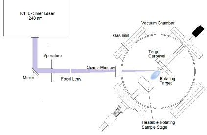
Thin films were deposited using the setup shown in Figure 2.1, with the following range of parameters:

 Laser energy 180–250mJ

 Energy density: 1–5 J/cm2

 Pulse rate: 6–10 Hz

 Substrate temperature range: 25 °C–700 °C

 Target → substrate distance: 3–6 cm

 Base vacuum pressure: ≤ 5 x 10-5

Torr

 Oxygen pressure: 0.5–200 mTorr

 Argon pressure: 0–100 mTorr

(35)

Characterization Techniques

2.3

2.3.1 X-Ray Diffraction (XRD)

XRD was done primarily using a PANalytical Empyrean multipurpose diffractometer featuring several interchangeable PreFIX modules. θ-2θ diffraction data for phase identification was recorded using a programmable divergence slit incidence beam optic with a 1/2 ° anti-scatter slit paired with an X’Celerater 1-D strip detector as the receiving optic. Epitaxial thin films were typically characterized using a double-bounce Ge hybrid monochromator as the incidence beam optic, while a 0.18 ° parallel plate collimator (PPC) with a Xe proportional counter was used as the receiving optic. Textured thin films were characterized using the hybrid optic paired with the 1-D strip detector or the PPC and proportional counter. Phase analysis was carried out using Highscore Plus, while epitaxial films were analyzed using Expert Epitaxy.

Diffraction experiments under non-ambient conditions were performed using a PANalytical Empyrean diffractometer equipped with a HTK-1200N stage, capable of heating to 1200 °C. θ-2θ scans were measured continuously as temperature was increased. Incident beam optics included a programmable divergence slit set to 1/32 °, with a 1/2 ° anti-scatter slit. This system is equipped with a PIXel1D detector.

2.3.2 Differential Scanning Calorimetry (DSC)

(36)

crucible type and should always be confirmed in the manual. In the case of Pt, standards used included AgS, BaCO3 and CsCl.

(37)

X-Ray Absorption Fine Structure (XAFS)

2.4

2.4.1 Sample Preparation

For transmission mode experiments, sample oxide powders were thoroughly mixed and pre-reacted at 1000 °C in air for 12-48 hours. Powder was checked for phase identification via XRD every 12 hours and remixed to promote a uniform reaction before being replaced in the furnace. The ESO powders were then milled to a fine grain, averaging less than 5m, using a SPEX 8000 Mixer/Mill.

It is critical that samples are prepared to meet the required thickness for 1 absorption length, defined as 1/µ, where µ is the absorption coefficient. The equation for calculating the absorption coefficient for a material is given by

𝜇 ≅ 𝜌 ∑ 𝜎

_𝑖𝑚𝑖 𝑀

𝑖

.

(2.1)

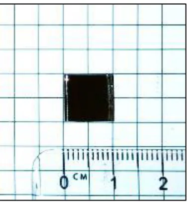
(38)

Figure 2.3 Photograph of EXAFS sample. Powder is evenly dispersed on Kapton tape, and folded three times to create a 1 cm x 1 cm square. Kapton is x-ray transparent, and the tri-fold creates the correct number of layers corresponding to appropriate sample thickness.

Table 2.1 Table of EXAFS scattering cross sections, absorption lengths, and calculated mass.

Energy 7709 8333 8979 9659

σMg 46.336 36.732 29.367 23.579

σCo 377.728 308.62 253.701 209.067

σCu 57.97 46.649 288.976 239.816

σNi 54.791 334.554 277.36 230.33

σZn 66.565 54.067 44.3 265.759

σO 12.563 9.895 7.875 6.306

ρ 6.128 6.128 6.128 6.128

σTotal 622.52 803.53 940.22 1039.73

(39)

2.4.2 XAFS Measurements

XAFS was measured at the Advanced Photon Source (APS) beamline 12-BM-B under general user proposals GUP-38672/GUP-40352 and beamline 10-BM-B under general user proposal GUP-46129.

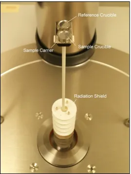
J14 powder samples were measured in transmission mode on 12-BM-B with an energy range of 7500 eV to 12000 eV, covering all absorber cations with the exception of Mg. A labeled photograph of the general setup for beamline 12-BM-B is shown in

Figure 2.4. Measurements on this beamline were performed using three sequential FMB Oxford – IC Plus 150mm ionization chambers, filled with 100% N2, labeled I0, I1,

and I2, respectively. The transmission sample, prepared in the way described in section

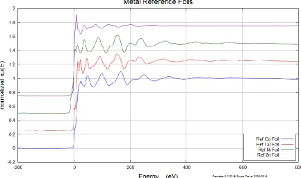
2.4.1, is located between chambers I0 and I1. All metal reference foils are provided by

EXAFS Materials [64], and the reference foil for a specific absorber is located between chambers I2 and I3. References used in transmission experiments include Co, Ni, Cu,

(40)

(41)

(42)

3 Entropy-Stabilized Oxides

Published in Nature Communications, 29 September (2015) DOI: 10.1038/ncomms9485

Christina M. Rost1, Edward Sachet1, Trent Borman1, Ali Moballegh1, Elizabeth C. Dickey1, Dong Hou1, Jacob L. Jones1, Stefano Curtarolo2, and Jon-Paul Maria1

1

Department of Materials Science and Engineering, North Carolina State University, Raleigh NC, 27695, USA

2

Department of Mechanical Engineering and Materials Science, Center for Materials Genomics, Duke University, Durham, NC 27708, USA

Abstract

3.1

(43)

Main Text

3.2

A grand challenge facing materials science is the continuous hunt for advanced materials with properties that satisfy the demands of rapidly evolving technology needs. The materials research community has been addressing this problem since the early 1900s when Goldschmidt reported the "the method of chemical substitution" [65], that combined a tabulation of cationic and anionic radii with geometric principles of ion packing and ion radius ratios. Despite its simplicity, this model enabled a surprising capability to predict stable phases and structures. As early as 1926 many of the technologically important materials that remain subjects of contemporary research were identified (though their properties were not known); BaTiO3, AlN, GaP, ZnO, and GaAs

are among that list.

These methods are based on overarching natural tendencies for binary, ternary, and quaternary structures to minimize polyhedral distortions, maximize space filling, and adopt polyhedral linkages that preserve electroneutrality [7], [65], [66]. The structure-field maps compiled by Muller and Roy catalogue the crystallographic diversity in the context of these largely geometry-based predictions[67]. There are, however, limitations to the predictive power, particularly when factors like partial covalency, and heterodesmic bonding are considered.

(44)

extensive ion substitution schemes [80], new 18-electron ABX compounds [81], and new ferroic semiconductors [82].

While these methods offer tremendous predictive power and an assessment of composition space intractable to experiment, they often utilize density functional theory calculations conducted at zero Kelvin. Consequently, the predicted stabilities are based on enthalpies of formation. As such, there remains a potential section of discovery-space at elevated temperatures where entropy predominates the free energy landscape.

This landscape was explored recently by incorporating deliberately five or more elemental species into a single lattice with random occupancy. In such crystals, entropic contributions to the free energy, rather than the cohesive energy, promote thermodynamic stability at finite temperatures. The approach is being explored within the high-entropy-alloy family of materials (HEAs) [31], in which extremely attractive properties continue to be found [40], [83]. In HEAs, however, discussion remains regarding the true role of configurational entropy [84]–[87], as samples often contain second phases, and there are uncertainties regarding short range order. In response to these open discussions, HEAs have been referred to recently as multiple-principle-element alloys [88].

(45)

transitions, normal materials melt, however, it is conceivable that synthetic formulations exist that exhibit them.

Inspired by research activities in the metal alloy communities and fundamental principles of thermodynamics we extend the entropy concept to five-component oxides. With unambiguous experiments we demonstrate the existence of a new class of mixed oxides that not only contains high configurational entropy, but is indeed truly entropy-stabilized. Additionally, we present a hypothesis suggesting that entropy-stabilization is particularly effective in a compound with ionic character.

3.2.1 Results

3.2.1.1 Choosing an appropriate experimental candidate

The candidate system is an equimolar mixture of MgO, CoO, NiO, CuO, and ZnO, (which we label as “J14”) so chosen to provide the appropriate diversity in structures, coordination, and cationic radii to test directly the entropic ansatz. The rationale for selection is as follows: the ensemble of binary oxides should not exhibit uniform crystal structure, electronegativity, or cation coordination, and there should exist pairs, e.g., MgO-ZnO and CuO-NiO, that do not exhibit extensive solubility. Furthermore, the entire collection should be isovalent such that relative cation ratios can be varied continuously with electroneutrality preserved at the net cation to anion ration of unity. Tabulated reference data for each component, including structure and ionic radius, can be found in Supplementary Table 3.1.

3.2.1.2 Reversibility

(46)

are depicted in Figure 3.1. After 700 °C, two prominent phases are observed, rocksalt and tenorite (monoclinic structure). The tenorite phase fraction reduces with increasing equilibration temperature. Full conversion to single-phase rocksalt occurs between 850 °C and 900 °C, after which there are no additional peaks, the background is low and flat, and peak widths are narrow in two-theta (2𝜃) space.

Reversibility is a requirement of entropy-driven transitions. Consequently, low temperature equilibration should transform homogeneous 1000 °C-equilibrated J14 back to its multiphase state (and vice versa upon heating). Figure 3.1 also shows a sequence of XRD patterns for such a thermal excursion: initial equilibration at 1000 °C, a second anneal at 750 °C, and finally a return to 1000 °C. The transformation from single-phase to multi-phase to single-phase is evident by the x-ray patterns and demonstrates an enantiotropic (i.e., reversible with temperature [91]) phase transition.

(47)

3.2.1.3 Testing entropy though composition variation

A composition experiment is conducted to further characterize this phase transition to the random solid solution state. If the driving force is entropy, altering the relative cation ratios will influence the transition temperature. Any deviation from equimolarity will reduce the number of possible configurations Ω (Sc = kB lnΩ), thus increasing the

transition temperature. Because Sc (xi) is logarithmically linked to mole fraction via ~xi

ln(xi), the compositional dependence is substantial.

This dependency underpins our gedankenexperiment where therole of entropy can be tested by measuring the dependency of transition temperature as a function of the total number of components present, and of the composition of a single component about the equimolar formulation.

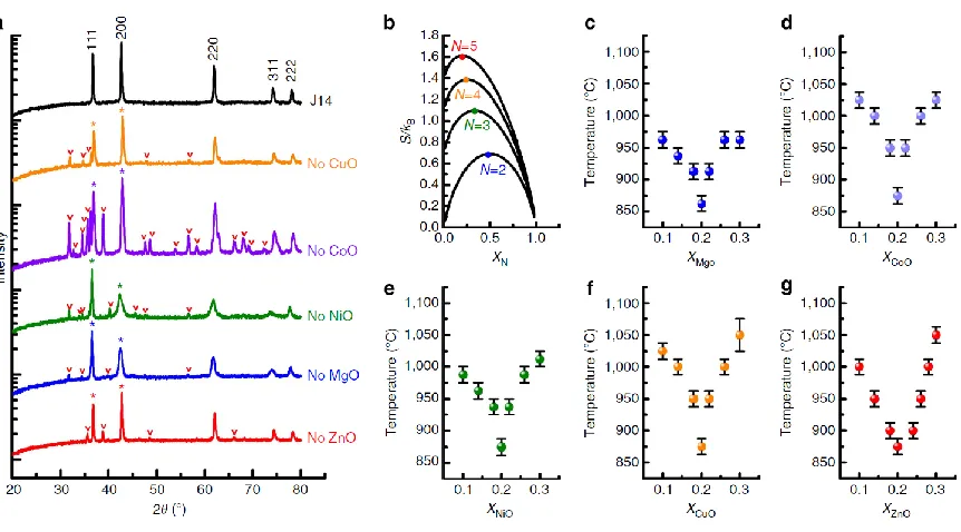
The calculated entropy trends for an ideal mixture are illustrated in fig. 2(b), which plots configurational entropy for a set of mixtures having N species where the composition of an individual species is changed and the others (N-1) are kept equimolar. Two dependencies become apparent: the entropy increases as new species are added and the maximum entropy is achieved when all the species have the same fraction. Both dependencies assume ideal random mixing. Two series of composition-varying experiments investigate the existence of these trends in formulation J14.

(48)

The second experiment uses five individual phase diagrams to explore the configurational entropy versus composition trend. In each, the composition of a single component is varied by ±2%, ±6% and ±10% increments about the equimolar composition while the others are kept even. Since any departure from equimolarity reduces the configurational entropy, it should increase transition temperatures to single phase, if that transition is in fact entropy driven. The specific formulations used are given in Supplementary Table 3.2.

Figure 3.2 (c-g) are phase diagrams of composition versus transformation temperature for the five sample sets that varied mole fraction of a single component. The diagrams were produced by equilibrating and quenching individual samples in 25 °C intervals between 825 °C and 1125 °C to obtain the Ttrans-composition solvus. In all cases

equimolarity always leads to the lowest transformation temperatures. This is in agreement with entropic promotion, and consistent with the ideal model shown in Figure 3.2 (b). One set of raw x-ray patterns used to identify Ttrans for 10% MgO is given as an

(49)

(50)

3.2.1.4 Testing endothermicity

R

eversibility and compositionally-dependent solvus lines indicate an entropy driven

process. As such, the excursion from multi-phase to single-phase should be endothermic. An entropy-driven solid-solid transformation is similar to melting, thus requires heat from an external source [92]. To test this possibility, the phase transformation in formulation J14 can be co-analyzed with differential scanning calorimetry and in-situ temperature dependent x-ray diffraction using identical heating rates. The data for both measurements are shown in Figure 3.3. Figure 3.3 (a) is a map of diffracted intensity versus diffraction angle (abscissa) as a function of temperature. It covers approximately 4 degrees of 2θ- space centered about the 111 reflection for J14. At a temperature interval between 825 °C and 875 °C, there is a distinct transition to single-phase rocksalt structure –all diffraction events in that range collapse into an intense (111) rocksalt peak.

(51)

(52)

3.2.1.5 Testing homogeneity

All experimental results shown so far support the entropic stabilization hypothesis. However, all assume that homogeneous cation mixing occurs above the transition temperature. It is conceivable that local composition fluctuations produce coherent clustering or phase separation events that are difficult to discern by diffraction using a laboratory sealed tube diffractometer. The solvus lines of Figure 3.2(c-g) support random mixing, as the most stable composition is equimolar (a condition only expected for ideal/regular solutions), but it is appropriate to ensure self-consistency with direct measurements. To characterize the cation distributions, extended x-ray absorption fine structure (EXAFS) and scanning transmission electron microscopy with energy dispersive x-ray spectroscopy (STEM EDS) is used to analyze structure and chemistry on the local scale.

(53)

(54)

As a corroborating measure of local homogeneity, chemical analysis was conducted using a probe-corrected FEI Titan STEM with EDS detection. Thin film samples of J14, prepared by pulsed laser deposition, are the most suitable samples to make the assessment. Details of preparation are given in the methods, and x-ray and electron diffraction analysis for the film are provided in Supplementary Figure 3.10 and Figure 3.11. The sample was thinned by mechanical polishing and ion milling. Figure 3.5 shows a collection of images including 5(a), the high-angle annular dark field signal (HAADF).

(55)

Figure 3.5 STEM-EDS analysis of J14. (a) is a HAADF image. Panels labeled as Zn, Ni, Cu, Mg and Co are intensity maps for the respective characteristic x-rays. The individual EDS maps show uniform spatial distributions for each element and are atomically resolved.

(56)

3.2.2 Discussion

The set of experimental outcomes show that the transition from multiple-phase to single-phase in J14 is driven by configurational entropy. To complete our thermodynamic understanding of this system, it is important to understand and appreciate the enthalpic penalties that establish the transition temperature. In so doing, the data set can be tested for self-consistency, and the present data are brought into the context of prior research on oxide solubility.

First we consider an equation relating the initial and final states of the proposed phase transition:

MgO(RS)+NiO(RS)+CoO(RS)+CuO(T)+ZnO(W) = (Mg,Ni,Co,Cu,Zn)O(RS) (3.1)

(57)

This assumption is consistent with the report of Davies et al., who showed that the chemical potential of a particular cation in a particular structure is associated with the molar volume of that structure. Since the rocksalt phases of ZnO and CuO have molar volumes comparable to J14, their reference transition enthalpy values are considered suitable proxies.

In comparison, the maximum theoretically expected configurational entropy difference at 875 °C (the temperature were we observe the transition experimentally) between the single species and the random five-species solid solution is ~15 kJ/mol, 5 kJ/mol larger than the calculated enthalpy of transition. It is possible that the origins of this difference are related to mixing energy as the reference energy values for structural transitions to rocksalt do not capture that aspect.

While the present phase diagrams that monitor Ttrans as a function of composition

demonstrate rather symmetric behavior about the temperature minima, it is unlikely that mixing enthalpies are zero for all constituents. Indeed, literature reports show that enthalpies of mixing between the constituent oxides in J14 are finite and of mixed sign, and their magnitudes are on the same order as the 5 kJ/mol difference between our calculated predictions [95]. This energy difference may be accounted for by finite and positive mixing enthalpies.

Following this argument, we can achieve a self-consistent appreciation for the entropic driving force and the enthalpic penalties for solution formation in J14 by considering enthalpies of the associated structural transitions and expected entropy values for ideal cation mixing.

(58)

uncertainty of ± 2 kJ/mol). While we acknowledge the challenge of quantitative calorimetry, we note that this experimental result is intermediate to and in close agreement with the predicted values.

Compared to metallic alloys, the pronounced impact of entropy in oxides may be surprising given that on a per/atom basis the total disorder per volume of an oxide seems be lower than in a high-entropy-alloy, as the anion sublattice is ordered (apart from point defects). The chemically uniform sublattice is perhaps the key factor that retains cation configurational entropy. As an illustration, consider a comparison between random metal alloys and random metal oxide alloys.

Begin by reviewing the case of a two-component metallic mixture A-B. If the mixture is ideal, the energy of interaction EA-B = (EA-A + EB-B)/2, there is no enthalpic preference for

bonding, and entropy regulates solution formation. In this scenario, all lattice sites are equivalent and configurational entropy is maximized. This situation, however, never occurs as no two elements have identical electronegativity and radii values. Fig. 6(a) illustrates a two component alloy scenario A-B where species B is more electronegative than A. Consequently, the interaction energies EA-A, EB-B, and EA-B, will be different. A

random mixture of A-B will produce lattice sites with a distribution of first near neighbors, i.e., species A coordinated to 4-B atoms, 2-A and 2-B atoms, etc. Different coordinations will have different energy values and the sites are no longer indistinguishable. Reducing the number of equivalent sites reduces the number of possible configurations and S.

(59)

disorder perspective, if each cation lattice site is identical, and thus energetically similar to all others, the number of microstates possible within the macrostate will approach the maximum value.

Figure 3.6 A binary metallic compared to a ternary oxide. A schematic representation of two lattices illustrating how the first near-neighbor environments between species having different electronegativity (the darker the more negative charge localized) for (a) a random binary metal alloy, and (b) a random pseudo-binary mixed oxide. In the latter, near-neighbor cations are interrupted by intermediate common anions.

(60)

and the need for a rigorous theoretical exploration. It is presented currently as a possibility and suggestion for future consideration and testing.

We demonstrate that configurational disorder can promote reversible transformations between a multi-phase mixture and a homogeneous solid solution of five binary oxides, which do not form solid solutions when any of the constituents are removed. The outcome is representative of a new class of materials called “entropy-stabilized oxides.” While entropic effects are known for oxide systems, e.g., random cation occupancy in spinels [89], order-disorder transformations in feldspar [97], and oxygen non-stoichiometry in layered perovskites [98], the capacity to actively engineer configurational entropy by composition, to stabilize a quinary oxide with a single cation sublattice, and to stabilize unusual cation coordination values is new. Furthermore, these systems provide a unique opportunity to explore the thermodynamics and structure-property relationships in systems with extreme configurational disorder.

Experimental efforts exploring this composition space are important considering that such compounds will be challenging to characterize with computational approaches minimizing formation energy (e.g., genetic algorithms) or with ad-hoc thermodynamic models (e.g., CALPHAD, Cluster Expansion) [6].

(61)

3.2.3 Methods

3.2.3.1 Solid-state synthesis of bulk materials

MgO (Alfa Aesar 99.99%), NiO (Sigma Aldrich 99%), CuO (Alfa Aesar 99.9%), CoO (Alfa Aesar 99%) and ZnO (Alfa Aesar 99.9%) are massed and combined using a shaker mill and 3 mm diameter yttrium-stabilized zirconia (YSZ) milling media. To ensure adequate mixing, all batches are milled for at least two hours. Mixed powders are then separated into 0.500 g samples and pressed into 1.27 cm diameter pellets using a uniaxial hydraulic press at 31,000 N. The pellets are fired in air using a Protherm PC442 tube furnace.

3.2.3.2 Temperature evolution of phases

(62)

receiving slits to ensure constant illumination area, a Ni filter, and a 1-D 256 element strip detector. The samples are placed in a resistively heated HTK-1200N hot stage in air. The samples are ramped at a constant rate of 5 °C/min with a theta-two theta pattern captured every 1.5 minutes. Calorimetry data are collected using a Netzsch STA 449 F1 Jupiter system in a Pt crucible at 5 °C/min in flowing air.

3.2.3.3 Determining solvus lines

Five series of powders are mixed where the amount of one constituent oxide is varied from the parent mixture J14. Supplementary Table 3.2 List of compositions used to prepare the transition temperature phase diagrams in Figure 3.2(c-g) in the main text.lists the full set of samples synthesized for this experiment. Each individual sample is cycled through a heat-soak-quench sequence at 25 °C increments from 850 °C up to 1150 °C. The soak time for each cycle is 2 hours, and samples are then quenched to room temperature in less than 1 minute.

(63)

reproducibility, it is completed a second time using shorter increments and 25 °C anneals. Findings in both sets are identical to within experimental error bar values. In the latter case, error bars correspond to the annealing interval value of 25 °C.

In the main text relating to Figure 3.2(a) we note that in addition to small peaks from second phases, x-ray spectra for N=4 samples with either NiO or MgO removed show anisotropic peak broadening in 2θ and skewed relative intensities where I(200)/I(111) is

less than unity. This ratio is not possible for the rocksalt structure. Supplementary Table 3.3 shows the result of calculations of structure factors for a random equimolar rocksalt oxide with composition J14. Calculations show that the 200 reflection is the strongest, and that the experimentally measured relative intensities of 111/200 are consistent with calculations. We use this information as a means to best assess when the transition to single phase occurs since the most likely reason for the skewed relative intensity is an incomplete conversion to the single-phase state. This dependency is highlighted in Supplementary Figure 3.7 Expanded view of one XRD temperature ladder showing the progression to single phase with 25 °C annealing steps. Red arrows indicate second phases,

green and blue arrows indicate shoulders of second phases associated with wurtsitic and

rocksalt structures respectively. Dashed lines highlight relative intensity values. Note that for

rocksalt, I111 cannot be larger than I200, thus we can use the relative intensity values as a

co-indicator of the final transition to single phase.

3.2.3.4 X-ray absorption fine structure (XAFS)

(64)

incident x-ray energies equal to or greater than their respective binding energies. The emitted photoelectron wave interacts with neighboring species, and the resulting absorption spectrum, displayed as absorption intensity versus incident energy, shows characteristic modulations unique to the target atom and its environment.

Equimolar amounts of the constituent oxides (MgO, NiO, CuO, CoO, and ZnO) are mixed and pre-reacted at 1000 °C in air for 12 hours with intermittent stirring during calcination. The product is mixed into an isopropyl alcohol slurry and ball milled using YSZ media for 24 hours. The powder is then dried in a fume hood at room temperature then re-fired at 1000 °C for 12 hours, then checked via x-ray diffraction to ensure phase purity and that peaks remain narrow and intense. Milled grain size is measured using scanning electron microscopy and determined to average ~10 microns.

A 2:1 powder to 10%PVA/H2O suspension is mixed continuously to disperse particles

within the solution as well as aid in breaking up any agglomerates. Using a Cookson Electronics P-6000 spin coater, thin layers are spun onto 2cm x 2cm square pieces of 25 micron thick Kapton. By trial and observation, it is determined that spinning at 2000 rpm for 1 minute makes a homogenous thin film with the appropriate quantity of particles for XAFS analysis.

(65)

measurement is repeated three times to check for systematic error and to improve signal to noise ratio.

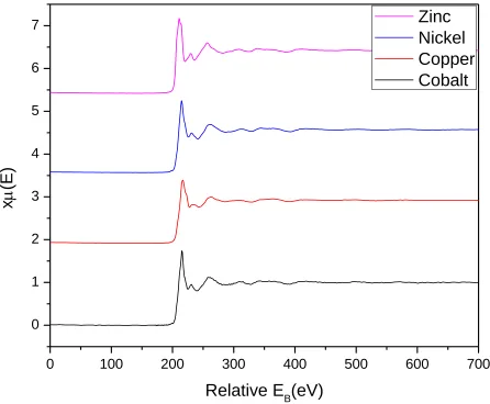
The raw data, shown in Supplementary Figure 3.9 plot the absorption edge and modulations on the post edge background. In order to isolate the EXAFS from these spectra, a background function is fit and subtracted. Energy space is transformed into k-space via the equation [24]:

k = √2m(E − E0)

ħ2 (3.2)

Where m is electron mass, ħ is the reduced Planck’s constant, and E0 is the absorption

edge energy. Supplementary Figure 3.9 Relative XAFS spectra as measured at APS beamline 12-BM after background normalization.shows the isolated EXAFS from the measurement. With this data, qualitative conclusions can be made pertaining to the degree of randomness of the cation species. If there were ordering within the system, these spectra would not demonstrate such consistent oscillatory structure and the scattering pathways for individual species would be unique. We limit our current conclusions at this somewhat conservative level as it provides the evidence needed to support a random solid solution.

3.2.3.5 Scanning Transmission Electron Microscopy

(66)

film sample was used for two reasons: 1) an edge-oriented substrate facilitates imaging along a low index zone axis perpendicular to the thinnest portion of the sample (this can be challenging for random powder specimens), and 2) by capping the thin film with a conductor, one can provide a conductive pathway to mitigate the sample charging that ultimately manifests in image drift. To do so, J14 films were coated with 50 nm of indium tin oxide at room temperature using RF-magnetron sputtering. Indium tin oxide is the preferred conductor as it is mechanically similar to a halide oxide and thus responds comparably to mechanical polishing.

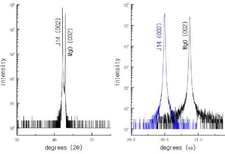
Laser-ablated samples were examined by 4-circle diffraction to assess crystallinity and epitaxy. Supplementary Figure 3.10 shows a theta-two theta and an omega scan for J14 prepared at 600 °C. The films are epitaxial to the MgO substrate (expected since the lattice mismatch is below 1%), and the mosaicity observed in the omega circle is consistent with that present in the MgO substrate. MgO substrates are known to have limited crystal quality (~0.02 ° in omega) due to the flame-fusion technique used to grow them.

An Allied Multiprep polishing system is utilized to prepare a cross-sectional electron microscopy sample by wedge polishing technique [100]. To achieve electron transparency, the polished sample is ion-milled with a Fischione Model 1050 Ion Mill while cooling with liquid nitrogen.

(67)

corresponding HAADF-STEM images in which the atomic columns containing heavier elements are observed brighter.

We note that STEM analysis is also performed on cryogenically fractured J14 powder samples and epitaxial thin films along [001] and [110] zone axes. In all cases STEM EDS analysis revealed no second phases and homogeneous and random elemental distributions within the J14 crystals. The STEM data featured in Figure 3.5 of the main text was chosen since the thin film configuration coated with a capping layer of ITO mitigated charging most effectively and allowed access to near atomic resolution with channeling conditions.

(68)

3.2.3.6 Configurational entropy in the ideal model

The following derivation describes the method to determine the composition dependence of configurational entropy shown in fig. 2(b) of the main text. An N-species system having composition {xi} has ideal entropy equal to:

S = −k_B∑ x_i N

i=1

log(x_i) (3.3)

The maximum S is reached at equicomposition xi = 1/N for each i, so:

Smax = -kB log (N). (3.4)

If only one species is varied, composition x1 = x for instance, while leaving the other N-1

species at equicomposition:

xi≠1 = 1−x

N−1 . (3.5)

The ideal entropy becomes:

S = −k_B[xlog(x) + (N − 1)_N−11−xlog (_N−11−x)] = −k_B[xlog(x) + (1 − x)log (_N−11−x)]. (3.6)

(69)

Acknowledgements

3.3

J-P.M., E.C.D., and C.M.R. acknowledge support from ARO under contract W911NF-14-0285. J-P.M. and C.M.R. acknowledge the Advanced Photon source (supported by proposal 38672) for access to synchrotron experiments. S.C. acknowledges partial support by DOD (ONR-MURI- N000141310635), DOE (DE-AC02-05CH11231, BES #EDCBEE), the Duke Center for Materials Genomics, and the aflowlib.org consortium. The Authors acknowledge the use of the Analytical Instrumentation facility at North Carolina State University who provided access to x-ray diffraction and electron microscopy facilities. AIF is supported by the State of North Carolina and the National Science Foundation. J-P.M. and C.M.R. acknowledge useful discussions with Dr. Sungsik Lee at the Advanced Photon Source regarding collection and interpretation of XAFS data.

Author Contributions

3.4

(70)

Supplementary Materials

3.5

Table 3.1 Initial oxide components in alloyJ14.*L denotes low spin, H denotes high spin. From R.D. Shannon and C.T. Prewitt, "Effective ionic radii in oxides and fluorides," Acta. Cryst., v. B25, p925, p. 5, 1969.

Binary Oxide

Structure (Space Group)

N Cation Radius (nm)

MgO Rocksalt (Fm-3m) 6 0.072

NiO Rocksalt (Fm-3m) 6 0.063

CoO Rocksalt (Fm-3m) 6 L-0.065 H-0.074*

CuO Tenorite (C 2/c) 4 0.073

Entropy-Stabilized Oxides: Explorations of a Novel Class of Multicomponent Materials.

Abstract

Dedication

Biography

Acknowledgements

Table of Contents

List of Tables

List of Figures

1

Introduction

Materials and Technology

1.1

An Alternative Approach to Materials

1.2

Development

Basic Thermodynamic Principles

1.3

∆𝐺(𝑇, 𝑃) = ∆𝐻(𝑇, 𝑃) − 𝑇∆𝑆(𝑇, 𝑃)

.

𝐴 + 𝐵 → 𝐴𝐵.

∆𝑆

= −𝑅 ∑ 𝑥

𝑙𝑛(𝑥

)

∆S

∆𝐻

= ∆𝐻

(𝑥

, 𝑥

) = 𝑎

𝑥

𝑥

∆𝐺

= ∆𝐻

(𝑥

, 𝑥

)

1

1

1

0

0

0



H

X

0

X

X



S



G

𝑆 = 𝑆(𝑇, 𝑃)

.

𝑑𝑆(𝑇, 𝑃) = (

)

𝑑𝑇 + (

)

𝑑𝑃

.

𝛿𝑄 = 𝑇𝑑𝑆

𝛿𝑄 = 𝑇 (

)

𝑑𝑇

.

𝛿𝑄 ≡ 𝐶

𝑑𝑇

.

𝑑𝑆 =

𝑑𝑇

.

Temperature, T

Gibbs Free Energy

G = H-TS

-+

Energy

Enthalpy, H

slope = Entropy, -S

𝑑𝐻 = 𝐶