ABSTRACT
MEHTA, VIRAJ KIRANKUMAR. Data fusion of multispectral remote sensing measurements using wavelet transform. (Under the direction of Dr. Hamid Krim.)
This thesis focuses on fusion of multispectral data available from remote sensing instruments. The aim is to develop fast and memory efficient algorithms that may be used for real-time implementation aboard satellites. Multiple channel data from the SSM/I instrument are used for experiments. Starting with a Bayesian estimation formulation of the data fusion problem, an attempt is made to take advantage of the sparseness resulting from wavelet transforms to optimize computational efficiency. After generating the necessary statistical models for the data to be estimated, a preconditioning whitening filter, which simplifies the choice of the required wavelet transform, is developed. The significant gains obtained by a compact representation in wavelet basis are shown. An input grid transformation leading to channel filters is then used to construct a real-time implementation of the optimal estimator. Simulated results of such a system are then used to demonstrate the achieved improvement in field resolution.
DATA FUSION OF MULTISPECTRAL REMOTE SENSING MEASUREMENTS USING WAVELET TRANSFORM
by
VIRAJ KIRANKUMAR MEHTA
A thesis submitted to the Graduate Faculty of North Carolina State University
in partial fulfillment of the requirements for the Degree of
Master of Science
ELECTRICAL ENGINEERING Raleigh, N.C.
April 2003
APPROVED BY:
Biography
Viraj Mehta was born on March 22, 1980 in Ahmedabad, India. He completed his
schooling at Prakash Higher Secondary School in May 1997. He graduated from Nirma
Institute of Technology (Gujarat University), Ahmedabad in May 2001 with a Bachelor of
Engineering degree in Electronics and Communications. His carried out his bachelor’s final
year project work at Physical Research Laboratory, Ahmedabad.
He then joined the Masters program in Electrical Engineering at North Carolina State
University, Raleigh, NC. There he was a part of the Vision, Information and Statistical Signal
Theories and Applications group (VISSTA), and worked on his thesis under the direction of
Dr. Hamid Krim. While working towards the master’s degree, he also spent summer and fall
Acknowledgements
I would like to express my sincere gratitude towards the guidance that I received from
my advisor Dr. Hamid Krim and thank him for being a mentor to me. Without him this thesis
would have but remained a dream. I would also like to thank the members of my advisory
committee, Dr. Brian Hughes and Dr. Marc Genton for their time and attention in evaluation
of the thesis. I would also like to thank Dr. Paul Fieguth for his insightful remarks and
comments.
It’s been an honor working in the Vision, Information and Statistical Signal Theories
and Applications (VISSTA) group. I am deeply thankful to Oleg V. Poliannikov and A. Ben
Hamza for their constant encouragement and motivation. I am also thankful to National
Aeronautics and Space Administration (NASA) for funding the research leading to my thesis.
My deepest gratitude goes to my parents and my sister, Maitri for their support, love
and encouragement. I thank them for their confidence in me that has helped me pull through
Table of Contents
List of Tables……….…… vi
List of Figures……… vii
1 INTRODUCTION ……….. 1
1.1 Motivation…….………..…….. ………... 1
1.2 The SSM/I Instrument……….. 2
1.3 Thesis Overview………... 5
2 PROBLEM FORMULATION FOR DATA FUSION………. 7
2.1 The Problem………. 7
2.2 Bayesian Estimation………. 8
2.3 Sparseness by Wavelet Transformation……… 9
2.4 Formulation for SSM/I………. 10
2.4.1 The Input Channels………. 10
2.4.2 The antenna gain operator……… 11
3 GENERATION OF STATISTICAL MODELS………... 14
3.1 Requirement……….………. 14
3.2 Estimating the covariance matrix P of X………. 14
3.2.1 Using statistics of 85V channel……… 14
3.2.2 Assumptions and procedures………... 15
3.2.3 Mathematical model……… 17
3.2.4 Generalization……….. 18
3.3 The covariance matrix for measurement errors……… 18
4 EXPERIMENTS AND OPTIMIZATIONS……….. 20
4.1 Direct method……… 20
4.2 Modification by a pre-whitening filter………. 22
4.3 Wavelet preconditioning………... 24
4.4 Comparison……….. 25
5 REAL-TIME IMPLEMENTATION………. 28
5.1 Input grid modification………. 28
5.2 MATLAB simulation experiment………. 31
5.2.1 Input grid modifier………... 31
5.2.2 Channel filter………... 34
5.2.3 Inverse wavelet transform ………... 35
5.2.4 Simulation result……….. 36
6 ADAPTING TO NON-STATIONARITY AND ERRORS……….. 38
6.1 Requirement………. 38
List of Tables
List of Figures
Fig. 1 SSM/I orbit and scan geometry from [4]………. 5
Fig. 2 Reformatting the input data………. 11
Fig. 3 The gain pattern for the 85V channel……….. 12
Fig. 4 A sample gain matrix for 85V………. 12
Fig. 5 Covariance Matrix for a row of 8 pixels along the scan direction for an 85V channel………... 16
Fig. 6 Fitting of the covariance to an exponential model……….. 16
Fig. 7 The final covariance matrix………. 17
Fig. 8 The estimation result of underlying field X from 4 input SSM/I channels using direct matrix computation……… 21
Fig. 9 Block representation of our estimation technique………... 22
Fig. 10 (a) the inverse filter matrix, (b) the impulse response of the whitening filter……... 23
Fig. 11 (a) The reformatted matrix and (b) its level-1 2D Haar wavelet decomposition… 24 Fig. 12 Pictorial description of the effect of the wavelet transform in 2-D………... 25
Fig. 13 Results of (a) direct method (b) with preconditioning……….. 26
Fig. 14 Frequency domain views of the 2-D versions of the (a) whitening filter and (b) the low frequency averaging Haar wavelet……….. 27
Fig. 15 The M matrix………. 29
Fig. 16 Pictorial representation of the input modification that leads to a representation of the matrix operator on the input as a filter………... 30
Fig. 17 Block Diagram representation of the real-time implementation of the optimal estimator………. 29
Fig. 18 The input grid modifiers for the (a) 85V channel and (b) 37V channel……… 33
Fig. 19 Impulse response of the 85V channel filter………... 34
Chapter 1
Introduction
1.1 Motivation
Remote sensing measurement instruments onboard satellites are increasingly complex
and many multi-channel and multi-sensor issues arise as a result. With an insatiable demand
for higher resolution, applications have led to an even greater number of channels, which in
turn was reflected by a deployment of a large number of sensors, with a daunting quantity of
data. From specifications [1] of most of these sensor instruments one can note the typical
features that they exhibit. Very recent and current multispectral and hyperspectral
instruments like the Multi-Spectral Scanner (MSS) & Thematic Mappers from the Landsat
missions, Advanced Spaceborne Thermal Emission and Reflection Radiometer (ASTER) &
Moderate Resolution Imaging Spectrometer (MODIS) onboard the Terra satellite, Hyperion
and Advanced Land Imager (ALI) instruments flown onboard the EO-1 satellite all indicate
the trend in satellite-based remote sensing to a greater number of channels with obvious
advantages. The information from these channels about vegetation, soil, rocks, oceans, air, is
invaluable to applications like vegetation mapping, mineral exploration, military use and
environmental conservation to name a few. Not only do the measurements at different
frequencies provide different information about different geological, atmospheric or even
useful enhanced resolution fields that represent all the information contained in the multiple
bands in a more compact form.
To comprehensively analyze this data while preserving all the original information,
one proceeds to achieve a coherent and composite image by way of clever sensor fusion. The
sheer size of the data, linearity in the physical models that relates measured data,
non-uniform spatial resolution, non-stationarity of the statistics of the data for global coverage
and missing data with errors are some of the major impediments in the path towards the goal
of efficient fusion. The myriad of applications of interest and constant emergence of new
ones has pushed towards using reprogrammable hardware for onboard satellite data
processing. This is to enhance flexibility and, most importantly, to reduce communication
burdens by limiting the extent to which raw, unprocessed data are transmitted to the ground.
It is thus essential to develop faster and more efficient data manipulation algorithms
compatible with FPGA implementations: algorithms using only basic and efficient
mathematical operations and very limited memory.
1.2 The SSM/I Instrument
The aim of this research work is to thus develop algorithms, which can be used to
generate higher resolution fields, while preserving information contained in all the different
sensor channels of an instrument. The Special Sensor Microwave/Imager (SSM/I) is in that
sense an adapted instrument that generates data consistent with our research goals, the results
of which may be used to evaluate our algorithms by comparing to more highly performing
The SSM/I is a passive microwave radiometer flown aboard Defense Meteorological
Satellite Program (DMSP) satellites. The SSM/I orbit is near circular, sun-synchronous, and
near polar, with an altitude of 860 km and an inclination of 98.8°. The orbital period is 102
minutes. This orbit provides complete coverage of the Earth, except for two small circular
sectors 2.4° centered on the North and South poles [2]. The SSM/I rotates continuously about
an axis parallel to the local spacecraft vertical and measures the upwelling scene brightness
temperatures. The absolute brightness temperature of the scene incident upon the antenna is
received and spatially filtered to produce an effective input signal or antenna temperature at
the input of a feedhorn antenna. The passive microwave radiometer output voltages are then
transmitted to the ground base stations.
SSM/I consists of seven channels, each of which may be considered as separate
total-power radiometers that simultaneously measure the microwave emission coming from the
Earth and the intervening atmosphere. Dual-polarization measurements are taken at 19.35,
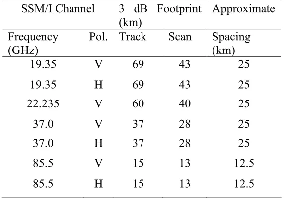
37.0, and 85.5 GHz, and only vertical polarization is observed at 22.235 GHz. Spatial
resolutions vary with frequency. Table 1 lists the frequencies, polarizations and temporal and
spatial resolutions of the seven channels.
Earth observations are taken during a 102.4° arc centered on the spacecraft sub track
in the aft direction and corresponds to a 1394 km wide swath, as shown in the figure 1.
During each scan, the 85 GHz channels are sampled 128 times over the 102.4° arc.
Observations at the lower frequencies are only taken every other scan and are sampled 64
times over the arc. This sampling pattern results in a 12.5 km pixel spacing at 85 GHz and a
25 km pixel spacing at the lower frequencies. Scans during which the lower channels are
The SSM/I data is well adapted to the goals of our research. It provides multiple
microwave channels that offer an opportunity for fusion to generate an enhanced resolution
field. The individual antenna gain patterns are different so that they can also be accounted
for. The spatial and temporal resolutions and patterns are different for some channels so that
they can be accounted for in the proposed models and help in development of real-time
algorithms that are to match the data acquisition rates. In addition, the statistics of the data
(as will be shown later) vary notably over global coverage. The use of SSM/I is an example
for proposing a common algorithm that is sufficiently generic to be applicable for other for
other measurement instruments.
SSM/I Channel 3 dB Footprint
(km)
Approximate
Frequency (GHz)
Pol. Track Scan Spacing (km)
19.35 V 69 43 25
19.35 H 69 43 25
22.235 V 60 40 25
37.0 V 37 28 25
37.0 H 37 28 25
85.5 V 15 13 12.5
85.5 H 15 13 12.5
TABLE I
SIZES OF THE 3-dB ANTENNA FOOTPRINTS AND THE APPROXIMATE SPACING OF THE MEASUREMENTS IN THE TRACK AND SCAN DIRECTIONS OF THE SSM/I CHANNELS (TAKEN
Fig. 1 SSM/I orbit and scan geometry from [4]
1.3 Thesis Overview
The work of this thesis has been organized into 7 chapters. The 1st chapter introduces
the reader to the framework for data fusion in remote sensing and provides an understanding
of the motivation behind this work and the reasons for selecting SSM/I data for experimental
purposes.
In the 2nd chapter we deal with the mathematical formulation of the data fusion
problem at hand. The rationale behind choosing a Bayesian estimation framework for fusion,
and tools such as the wavelet transform for optimizing the formulation is explained. An
overview of the size and statistical nature of the quantities we consider are also provided.
The 3rd chapter deals with statistical analysis of the captured SSM/I sample data to
propose a covariance model for the underlying high-resolution field. The finer details of the
assumptions, which led to the proposed covariance model, are explained in this, in addition
to extending the procedure to more recent instruments. A simple covariance model for
measurement errors is also proposed with emphasis on its use to customize weighting of
In the 4th chapter we first describe the experiments carried out with the basic
formulation. Then we carry out some mathematical manipulations to impose a pre-whitening
condition on the data to be estimated. We then show, how when combined with a simple 2-D
Haar wavelet transform it results in immense savings for memory and computational
complexity.
A real-time implementation of the above formulation is described in the 5th chapter.
We also explain our approach of using channel filters to represent the acquired data in a
common basis where fusion is carried out by a manipulation of coefficients. A MATLAB
simulation result for this implementation with a corresponding comparison to the previous
matrix-based computations is given.
Chapter 6 offers suggestions to develop methods to adapt the proposed algorithm with
ranging statistical parameters. The resulting additional computational costs of an adaptive
requirement are also explained. Finally, in chapter 7 we conclude with an outline of the
Chapter 2
Problem formulation for Data Fusion
2.1 The Problem
The first crucial assumption we make in formulating our data fusion problem is that
of linearity. We, basically model the measurement signal of the brightness temperatures as a
linear combination of the actual field and measurement errors. Consider the following
equation:
E GX
Y= + (1)
where, X denotes the underlying field being measured,
G denotes the Gain of the measurement antenna,
E denotes the measurement error, and
Y denotes the observed measurements.
Note that Y and X need to be clearly defined in terms of the actual data available and the
field we are attempting to estimate. G is the gain operator which captures the integration
process to yield the measurements. By taking Y to be all the data measurements available
from various channels of the same field, the inverse problem of determining X, then
2.2 Bayesian Estimation
The data fusion problem, as described earlier, assumes data from multiple antenna
channel measurements. Another way of stating it is to harness and combine all available
information from all channel measurements to generate a higher resolution field. Several
approaches have been proposed in this regard. The theory [5] is based on the fact that the
density of the satellite measurements is higher than the resolution of the instrument, which
means that it is possible to take advantage of over sampling to reconstruct a higher resolution
image from low-resolution data. Several techniques have been proposed for image
enhancement based on a matrix inversion method proposed by Backus and Gilbert [6]. These
techniques are based on finding a linear combination of the surrounding measurements to
yield images at higher spatial resolution than the original data. These algorithms require
matrix inversion at each pixel, which means excessive time requirements. BGI methods are
however adapted to noisy measurements by tuning parameters to trade off noise and
resolution. Other techniques were based on the theory of image reconstruction and
enhancement from noisy irregular samples using algebraic image reconstruction techniques
(ART) [7]. Different algorithms based on ART have been adapted [8] to address the problem
of resolution enhancement of the remotely sensed data. These adaptations include controlling
noise and compensating for the attenuation introduced by the aperture function (Antenna gain
function).
Our estimation approach here is Bayesian. Several assumptions are in order before
formulating the estimation problem. We can safely assume that the measurement error E is
assuming that Y and X are Gaussian distributed i.e. by limiting our analysis to second order
statistics and solving Eq. (1), we get the following estimation equation [9],
Y R G G R G P
Xˆ =( −1+ T −1 )−1 T −1 (2)
Where the only new term P is the a priori Covariance Matrix of X. While this seems to
yield a direct solution to the inversion problem, an accounting for the non-stationarity of the
measured field and for the nature of the data makes it nontrivial. For example, the
non-stationarity implies that Eq. (2) is valid for only local patches of data and that the inversions
are required to be carried out at virtually every pixel of the data. This and several other
problems are addressed as we focus on the specific formulation for SSM/I.
2.3 Sparseness by Wavelet Transformation
To gain an insight into how we plan to apply a wavelet transform for simplification in
our data structure, we proceed as follows. We first effectively precondition the estimation
problem using a wavelet transform W,
,
WX
X = (3)
leading to an estimated X:
, ) ( )) ( ) ( ) ((
ˆ WPWT 1 GWT TR1 GWT 1 GWT TR1Y
X= − + − − − (4)
With a judicious choice of a wavelet and application of a pre-whitening condition, as we later
show, a great simplification of the above equations results which in turn impacts the
computational costs of matrix calculations and inversions well adapted to FPGA
2.4 Formulation for SSM/I
2.4.1 The Input Channels
To specialize the formulation of field estimations to SSM/I, we carefully format them
in a vector Y. In all we have seven available data channels namely: 19V, 19H, 22V, 37V,
37H, 85V, and 85H GHz channels. Since each channel is from a 2-dimensional grid, the first
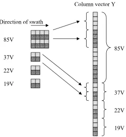
step is to vectorize this 2-D data into a 1-D column vector, i.e. Y85 =Vec[Y85]. We carry out simple vectorization and append various channel data to the same column vector data as
T 19 22 37
85, , , ]
[Y Y Y Y
Y= where Y85, Y37… are the vectorized measurements of each channel.
We determined that the mean of the data from different channels is different, and hence
proceeded to mean removal prior to fusion. In our experiments we only use the mean
removed vertical polarization channels at each frequency (four in all). Note that throughout,
it is required that the data come from a finite local patch of the underlying field with
stationary statistics. We also note that the size of the data coming from different channels is
different for the same local patch. Our goal is to generate an underlying field grid that is 4
times finer in resolution in both dimensions than the highest resolution channel available to
us (i.e. the 85GHz channels). Thus, for an NxN set of acquired data from 85V, we estimate
4Nx4N=16NxN pixels. The geometry of the measurements is such that the 19V, 22V and
37V channels are sampled at half the resolution (25km as opposed to 12.5 for 85V) and thus
for every 4 pixels that the 85V contributes the other channels contribute one pixel each in the
input data. This gives us a set of (NxN +3NxN/4)=7NxN/4 input data points. In Fig. 2 we
Fig. 2 Reformatting the input data
2.4.2 The antenna gain operator
To proceed with the formulation it is essential to model the antenna gain operator G.
According to Eq. (1), the G matrix operates on the underlying field X(size 16NxN column
matrix) to produce the measured data Y (size 7NxN/4 column vector as shown before). To
construct the required matrix G of size (7NxN/4) x (16NxN), we first model the individual
channel gains. For each of the four channels we assume a jointly binomial gain pattern. For
the sake of illustration, we consider the 85V channel. The geometry of the measurements
indicates that the 3dB footprint of the channels is 15km in length along the track and 13km in
length along the scan while there are measurements available 12.5 km in each of the two
directions. Thus, there exists a clear overlap between various measurements. Since for each 85V
37V
22V
19V 85V
37V
22V
19V
Direction of swath
85V measurement, we have an assumed 16 pixels of the underlying field X, the dimension
of each pixel in X is (12.5/4 x 12.5/4) = (3.125 x 3.125) km2. Now the actual footprint is
15km x 13km and thus approximately the gain pattern averages over a 6x4 patch of pixels of
X (taking 6 instead of 5 for generating a symmetric gain pattern will help simplify the
analysis later). Taking a jointly binomial gain pattern over this patch and after accounting for
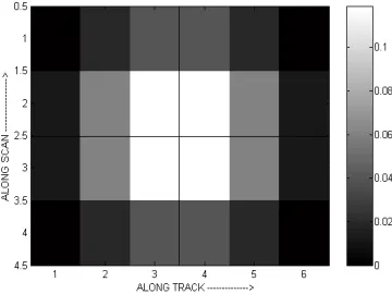
the approximations, we get the following pattern of Fig. 3.
Fig. 3 The gain pattern for the 85V channel (Note: overall gain is normalized to unity)
The above figure shows the gain pattern for a 2D patch of data. The same pattern
when made for a gain operator that converts a vectorized underlying field of 20x20 pixels
into a vectorized 85V measurement of 5x5 pixels is shown below in Fig. 4.
Fig. 4 A sample gain matrix for 85V
One can clearly note the overlap between 85V pixels by observing that some columns in the
above diagram have more than one non-zero row elements. This overlap is much more
evident for the lower frequency channels which have much larger footprints. It is thus clear
that there is considerable information in the channels, which may be exploited for estimating
a finer underlying field! The overall gain matrix G for all channels is again constructed by
appropriately combining individual gain matrices for all channels in correspondence to the
Chapter 3
Generation of statistical models
3.1 Requirement
To estimate the underlying field using Equation (2), we need to empirically estimate
the a priori covariance matrices P and R of the field X and the error in measurement E
respectively. The non-stationarity (non-homogeneity) of the measured field makes the
empirical estimation of P particularly challenging, and requires a careful evaluation of the
statistics of the available data. In accounting for the specific data formats, we develop an
analytical model which best reflects the empirical covariance statistics. In determining R,
some assumptions are made, and we in turn exploit that in weighting different measurement
channels.
3.2 Estimating the covariance matrix P of X
3.2.1 Using statistics of 85V channel
For estimating the covariance matrix of the underlying field we use the measurements
from the 85V channel. It is closest in terms of resolution to the underlying field than any of
the other channels. More importantly, the 85V channel is the channel in which the
Moreover, if we look at the gain pattern (footprint) of the 85V channel along the scan then
we observe that there is hardly any overlap in the scan direction. This is due to the width of
the footprint along the scan being 13km and the sampling rate in the same direction being
12.5 km. This is tantamount to saying that if we use the covariance behavior of the rows
along the scan direction, is such that its empirical estimate will be closest to the desired
model of the underlying field.
3.2.2 Assumptions and procedures
As detailed above, the estimation of the covariance matrix P is entailed in the
estimation of the covariance matrix for the 85V channel in the single dimension along the
scan. Recall that our initial formulation was assumed for a local patch of pixels. In other
words, the statistics may drastically vary for a different patch. The same problem is
encountered in the course of its empirical estimation, which thus requires that certain
procedures be adopted.
By way of experimentation on the 85V data sample we determined that if the global
mean is kept zero, then the covariance behavior is highly non-stationary. (This is the single
biggest challenge in obtaining the final model.) If we however, subtract the mean over local
patches in the entire grid of available data, then the resulting data has a stationary covariance
behavior. We develop an adaptive procedure for marching through the entire grid of data to
carry out the local mean removal namely “windowing”. For every single pixel in the entire
grid, we compute the mean of its neighboring values in a window of size 8x8. This mean is
then subtracted from the value of the pixel. This procedure achieves the “locally mean
The detrended data is subsequently used to estimate the covariance matrix of an
8-pixel row in the scan direction. The average over the entire field of available data is shown in
Fig. 5.
Fig. 5 Covariance Matrix for a row of 8 pixels along the scan direction for an 85V channel
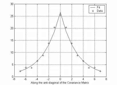
This covariance matrix has a very specific structure. If we in fact consider the anti-diagonal
of the above matrix it can then be shown to precisely fit an exponential model! Fig. 6 shows
the fitting of the data points from an anti-diagonal and a parallel diagonal (for greater points)
to the model
|) | exp( * )
(d A B d
C = (5)
with A = 26.5375 and B = -0.35398, where |d| is the distance between 2 pixels. We next
3.2.3 Mathematical model
Eq. (5) is generated for a row of data along the scan direction in the 85V channel.
Unlike the 85V the pixels in the underlying field suffer no overlap and their statistics can be
assumed isotropic. With this assumption it is straightforward to construct P. We need to
keep in mind the vectorization constraints imposed on the column vector for the formatted
underlying field. For a swath width N in terms of the underlying pixels one may see that P
has the following form.
= = ( ) )
,
(x y C d P
/
/
)2 (
/
/
)2(
( x N y N x x N y y N
C − + − − +
=
/
/
) (
/
/
) } (* exp{
* B x N y N 2 x x N y y N 2
A − − + − − +
= (6)
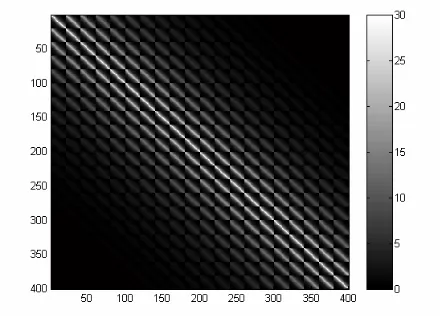
Note that the formulation of the problem for a patch of NxN pixels leads to this special
structure of the Covariance matrix. This basically means that since a pixel exhibits high
correlation with its neighbors, the covariance structure is high between not only adjoining
data points, but also between points at multiples of N because of the vectorization. For
example, observe the covariance matrix generated for a patch of 20x20 pixels, (i.e. of size
400x400) as shown in figure 7.
3.2.4 Generalization
Even though, the method outlined here for determining P is specific to the SSM/I
instrument, several key points may be generalized. For any given instrument, the
corresponding process would involve the following steps:
Observe characteristics of sample data to determine what input channel(s) provide
statistical data that is closest to the underlying field and thus has minimum
overlap.
Apply statistical modifications (e.g. local mean removal) to selected data to
guarantee the imposed assumptions of stationarity.
Compute the covariance matrix for the relevant input data points.
If possible, fit this covariance matrix with a mathematical model.
From the generated model, develop the final form that is adapted to the vectorized
field with a specified swath length.
3.3 The covariance matrix for measurement errors
The measurement error E in every channel is assumed to be zero mean additive
white gaussian noise. Assuming non-correlation and equal variance for one channel, the error
covariance matrix is just σ2I
for each of the channels, where σ is the standard deviation for
measurement errors in that channel.
We can have different error variances for different channels. Ideally, one would like
weighting factor. In other words, by selecting higher error variance for a particular channel
we are estimating our underlying field to a lesser extent from it. This turns out to be very
useful in the SSM/I setting. Since, the lower resolution channels give us less accurate
measurements then the higher ones, we might want to derive our estimation more from the
higher resolution channels than the lower ones. This leads us to selecting
2 85 2 37 2 22 2
19 σ σ σ
σ > > > where the terms are the measurement error variances of the respective
channels.
Note that this still does not provide us with an exact method to determine the
individual channel measurement error variances, but merely imposes constraints. We thus
have to empirically and a bit qualitatively select them. The final Covariance Matrix R is thus
diagonal with elements of the diagonal being the variance of the measurement error for the
channel that the measurement corresponds to, i.e.,
=
4 / 4 / 2 19 4 / 4 / 2 22 4 / 4 / 2 37 2 85 2 2 2 2 2 2 2 20
0
0
0
0
0
0
0
0
0
0
0
xn n xn n xn n xn nI
I
I
I
σ
σ
σ
σ
R
(7)Note that all the zeros in the above matrix indicate that there is no correlation
between measurement errors of various channels. Each of the individual error covariance
matrices for individual channels contributing to the above matrix is different in size. This is
due to the measured data for the underlying field which depends on n which is the width of
Chapter 4
Experiments and optimizations
4.1 Direct method
With the statistical models for the covariance matrices of the underlying field and of
the measurement error in place, we proceed to generate fusion results using direct but costly
matrix computations. We use Bayesian estimation Eq. (2), which, recall, is written as:
Y R G G R G P
Xˆ =( −1+ T −1 )−1 T −1
A sample experiment was carried out on a patch of data of size 10x10 pixels in the 85V
channel and 5x5 in the other channels. The corresponding size of the underlying field is thus
16 times that of the 85V channel, i.e. 40x40 pixels. Note that in the adopted format the X and
Y matrices are column vectors of size 1600 and 175 (100+25+25+25) respectively. The
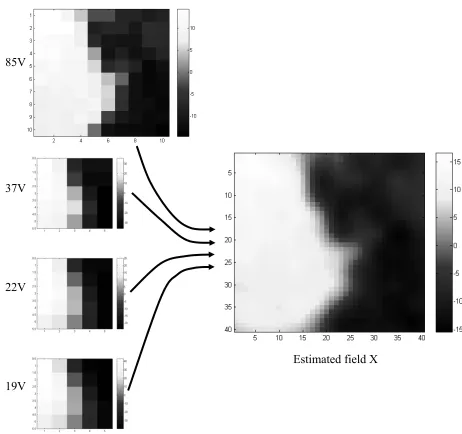
result is shown in Fig. 8.
A clear resolution improvement in the fusion based over the highest resolution
measured field is evident. While the optimality of this estimation method under the stated
assumptions is unquestionable, the computational cost is prohibitive. For a non-stationary
field with a varying covariance matrix the inversion (P−1+GTR−1G)−1, is required to be
performed for every stationary local patch. In general, without an adaptive algorithm this
would virtually mean inverting a 400x400 matrix twice at every pixel that needs to be
Fig. 8 The estimation result of underlying field X from 4 input SSM/I channels using direct matrix computation. The error variances are assumed to be 48, 36, 16, & 1 for the channels
19V, 22V, 37V & 85V respectively. 85V
Estimated field X
4.2 Modification by a pre-whitening filter
To simplify the analysis and improve the estimation technique, we proceed to
transform the measurements and hence the development. Clearly, in the process of estimating
the underlying field X, we have two sources of information: one that is based on the prior
knowledge of the statistical nature of the field and the other being the real time information
available as the data is acquired. One way of estimating the field X could be to combine this
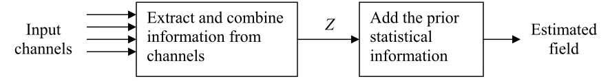
information in two sequential data processing blocks as shown in Fig. 9.
Fig. 9 Block representation of our estimation technique
From this perspective, the intermediate quantity Z in the estimation procedure is free of the
prior covariance statistics P and is thus white.
The key to partitioning the estimation process into two such blocks thus lies in
applying a preconditioning transform that makes the estimated field white. We obtain this
preconditioning transform by taking the Cholesky Factorization of the a priori covariance
matrix of X, i.e. P=AAT where A is a full rank Upper Triangular matrix. Now, letting
1 W
−
=A
F and rewriting the problem statement yields:
E X F GF
Y= − +
W 1
W (8)
Defining, 1
W W
−
=GF
G we get the Bayesian estimate of the quantity FWXas:
Y R G G R G I X F
X T 1
W 1 W 1 T W W
W ˆ ( )
ˆ = = + − − − (9)
Extract and combine information from channels
The above equation is exactly same as Eq. (2) except that the Gain matrix has now changed
and the prior on the estimated field is now an identity matrix, making it statistically white!
Note that this whole procedure requires the first block in Fig. 9 to restructure the covariance
statistics of the input channels, which are subsequently fused. This suggests the possibility of
further simplifying the first block by distinguishing the decorrelation and fusion steps as
further detailed in the next chapter.
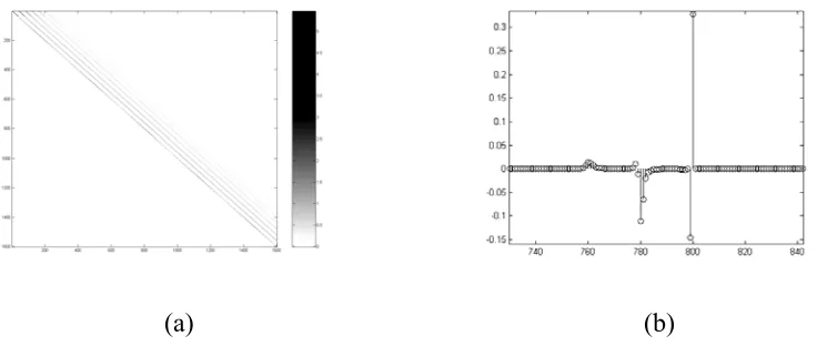
The matrix FW is in effect a whitening filter. Fig. 10 shows the structure of the
inverse filter matrix with the corresponding impulse response of the whitening filter on the
right. Closer observation of Fig. 10(b) reveals the short and long term dependency of a pixel
on the neighboring pixels in the same scan and the adjoining scans respectively. Note that in
practice we never use the whitening filter, and hence the inverse of the cholesky factorization
never needs to be computed. We only use 1 W
−
F (i.e. A) to “recolor” the estimated quantity
W
ˆ
X as the final step in the estimation process.
(a) (b)
4.3 Wavelet preconditioning
As indicated earlier, we plan on conquering the daunting computational burden by
taking advantage of sparseness resulting from wavelet transform. With the pre-whitening
condition imposed, the choice of a suitable wavelet for doing this becomes easier. In our
experiments, we carried out wavelet decomposition of the estimated quantity
W
ˆ
X (reformatted as 2-D image) using a 2-D Haar wavelet. We have experimentally
established that the only significant coefficients are the low frequency averages at the first
level. The remaining coefficients are all close to zero and may hence be thresholded.
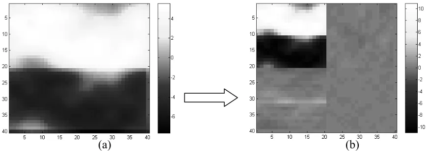
(a) (b)
Fig. 11 (a) The reformatted matrix XˆW and (b) its level-1 2D Haar wavelet decomposition.
This amounts to saying that an application of a wavelet transform Wl to the vectorized white
data XˆW will extract the low frequency portion (normalized averages of 4 adjoining pixels)
and preserve most of the information while reducing the size of data by a factor of 4.
Mathematically, defining Xl =WlXW, and Gl =GWWlT we can write the modified
estimation equation as:
Y R G G R G I X F W
X T 1
l 1 l 1 T l W l
l ˆ ( )
W
ˆ
X WlXˆW
Fig. 12 Pictorial description of the effect of the wavelet transform in 2-D
With these definitions in place, the estimation of the underlying field is a two-step process as
originally envisioned in Fig. 9, the first step entailing the estimation of the quantity Xˆl by
means of fusion of the input data channels using Eq. (10), and the second effecting the
reconditioning of the estimated quantity by applying an inverse wavelet transform followed
by an inverse whitening filter. The appeal of this technique lies in the fact that the
intermediate quantity Xˆl is represented in a compact wavelet basis. This has multiple
advantages. From a real-time FPGA implementation viewpoint, the size reduction of the
matrices Xl and Gl by a factor of 4 in one dimension and smaller size of (a factor of 4 in
both dimensions) the inversion 1
l 1 T
l )
(I+G R−G − provides a significant gain. This leads to
great savings in memory and computational time. Moreover, considering the case of an
onboard satellite implementation, it makes sense to decrease the communication burdens by
representing the estimated data in a compact form. This is again achieved by the wavelet
transformation if we carry out the necessary reconditioning filtering at ground base stations.
4.4 Comparison
For the same input data as described in Section 4.1, we now show estimation results
now of size 400x1(20x20) and the equivalent antenna gain matrix Gl is 175x400 instead of
the earlier 1600x1 and 175x1600 respectively. We have eliminated the necessity for inverting
the a priori covariance matrix P and the only significant inversion is that of the matrix
)
( T 1 l
l R G
G
I+ − which is of size 400x400 instead of the earlier 1600x1600. This is at a cost of
computing Gl, which may be taken care of offline and hence at a very minimal additional
cost.
(a) (b)
Fig. 13 Results of (a) direct method (b) with preconditioning
The above figure shows the results of the two methods side by side for comparison.
Except for some border effect pixels that are introduced because of the nature of the inverse
whitening filter, the two methods yield near exact estimation results. The achieved
simplifications are also justified from a frequency domain viewpoint. A field typically
contains high low-resolution information and low high-resolution information. By imposing
the pre-whitening condition our modified field is white meaning that the high frequency
components are emphasized. The reduction of coefficients by application of the Haar wavelet
(a) (b)
Fig. 14 Frequency domain views of the 2-D versions of the (a) whitening filter and (b) the low frequency averaging Haar wavelet. Note how the high frequency de-emphasis of the
Chapter 5
Real-time implementation
5.1 Input grid modification
We now proceed to develop a real-time implementation of the optimized estimation
formulation. Looking back at Fig. 9, it is the clear that the focus of the work here is to
develop a real-time implementation for the first block, since the second is already in the form
of a cascade of the inverse wavelet and inverse whitening filters. As was briefly discussed in
Chapter 4, there exists the possibility of simplification of the first block into de-correlation
and combination sub-blocks. The need for de-correlation of input channels arises from the
fact that the intermediate quantity to be estimated is white, and the combination is just a
restatement of fusion.
To visualize the intuition behind the following manipulations aimed towards
achieving a real-time implementation, consider the matrix representation of the first block,
i.e. T 1
l 1 l 1 T l ) ( + − − −
= I G R G G R
M . The estimation of the intermediate quantity is then just a
multiplication of the input with this matrix, i.e. Xˆl=MY and the final estimation is achieved
by reconditioning this intermediate quantity, i.e. T l
l -1
W ˆ
ˆ F W X
X= . Fig. 15 shows the M
matrix for input restricted to the 85V and 37V channels. (Note: Throughout this chapter we
use the 85V and 37V channels only for experimental purposes. Extension to other channels is
Fig. 15 The M matrix
The dimensions of the M matrix shown above are 400x125 for 400 pixels to be
estimated for a final field of 1600(40x40) pixels. The first 100 columns indicate operation on
the 100 input pixels from a 10x10 field in the 85V channel while the remaining 25 indicate
operation on the 25 input pixels from a corresponding 5x5 field in the 37V channel. Thus, the
first important conclusion is that we can separate the contributions to a pixel from various
input channel as follows:
[
M85 M37 ...]
M= (11)
where ,...M85,M37 correspond to different channels.
The estimation statement follows as:
MY Xˆl =
[
]
...... .
... 37 85 85 37 37
85
37
85 = + +
= Y M Y M Y
Y M
This implies that the operators M85,M37,... can individually de-correlate the input channels,
and the estimation of the intermediate preconditioned quantity is then just the addition of the
corresponding coefficients for each pixel in the adopted wavelet basis. Let’s now consider
the portion for the 85V channel first, i.e. the first 100 columns or M85. We notice a certain
pattern here. Looking at sets of 10 columns, each column in a set is a vertical shift of its
adjoining column by 2 pixels and each set is a vertical shift of the adjoining column by 20
(2x(Swath width)) pixels (one swath is 10 pixels here, since we are estimating from a 10x10
field of the 85V channel). It is now easy to see that our aim of developing a real-time
implementation is realized if we carry out some input reformatting that makes every column
a vertical shift of the adjoining column by one pixel, i.e. construct a matrix filter to achieve
such shifts. This is easily most efficiently accomplished by effectively increasing the 85V
channel input sampling rater (to a higher resolution grid corresponding to the quantity to be
estimated) by a systematic insertion of zeros. This is pictorially shown in Fig. 16.
Fig. 16 Pictorial representation of the input modification that leads to a representation of the matrix operator on the input as a filter.
A similar grid modification is required for the 37V channel. Given its original lower
sampling rate, more zeros are required for it as the 37V channel. With each M matrix as a
modified from Y85,Y37,... to Z85,Z37,... by the aforementioned technique. Now the matrices
,... , 37 85 M
M become ,...F85,F37
.... 37 37 85 85
l= + +
∴X F Z F Z
.... 37 37 85 85
l= ∗ + ∗ +
∴X f Z f Z where * are convolution (13)
Thus, Xlis obtained by filtering Z85,Z37,... by the filters F85,F37,... and adding up the output
coefficients. The simplification of the M matrix into a bank of filters thus completes the
real-time implementation of the optimal estimator.
5.2 MATLAB simulation experiment
We now proceed to show the exact construction of the real-time implementation. Fig.
17 shows the block diagram representation of such a system. It can easily be extended to
include additional channels using a similar approach. On the left hand side is what might be
called a bank of filters for the channels. An “input reformatting” block, which carries out the
input grid modification as previously explained, precedes every channel filter. The outputs of
the various channel filters are added after accounting for synchronization delays. The sum is
then the conditional estimate of the field of interest. The inverse wavelet and “re-coloring”
filters applied to this sum yield the final estimate as shown on the right hand side of the block
diagram. We now explain in detail the construction of each individual block.
5.2.1 Input grid modifier
Let’s take the input grid modifier of the 85V channel as an example. Fig. 18 (a)
32
insertion of one zero between every two pixels. The pixels corresponding to one swath are
then buffered and appended by an equal number of pixels of value zero that form an entire
zero swath. This is now unbuffered to produce the grid-modified input. For the 37V channel,
the process is similar and is shown in Fig 18 (b).
(a)
(b)
5.2.2 Channel filter
We again take as an example the construction of the 85V channel filter. The first step
is to obtain a column of the M85matrix, which defines the impulse response of the required
filter.
Fig. 19 Impulse response of the 85V channel filter.
We can easily construct a Direct Form I FIR filter with the given coefficients of the impulse
response. Even though the column length is 400 for our example, the number of significant
values in the impulse response is much smaller, and the resulting filter hence has a compact
form. To make the filter independent of the swath width, a crucial observation is in order,
namely that the impulse response has significant values in sets of points equivalent to a swath
width. The zero values coincide with the middle of any two consecutive sets. This is
basically just indicative of the short and long-range dependence of the acquired data on the
pixels in the underlying field. For our filter design to be valid for any swath width, we just
need to insert zero points between the sets such that the width of the swath still corresponds
between parallel forward paths of the FIR filter. The construction of filters for other channels
is similar.
Fig. 20 A section of the Direct Form 1 implementation of the channel filter for 85V channel. (Note the intermediate integer delays dependent on swath width.)
5.2.3 Inverse wavelet transform
The construction of the re-coloring filter is exactly the same as that of the channel
filter, as it also needs care in accommodating the swath width in its structure. The only
remaining block is the inverse Haar wavelet transform and is shown in Fig. 21. The
multiplicative factor 0.5 occurs because of power normalization. The rest is a process of
generating the entire 2D image from the available low frequency average. This just requires a
four-field replication of the pixel value, first two times in a row and then a replication of an
entire row corresponding to a swath. The buffering and unbuffering shown, is required to
Fig. 21 Implementation of the inverse Haar wavelet transform for vectorized 2D data.
5.2.4 Simulation result
We now show the MATLAB simulation result of the real-time implementation with
an 85V channel data size of 256x128 pixels resulting for an estimated data size of 1024x512
= 219 pixels! This is shown in Fig. 22 along with an inset of a smaller size of data to note the
improvement in resolution. While the estimation of the inset data seems flawless one can
notice some boundary value problems in the estimated image. This is mainly because of the
dependence of the rightmost pixels on the leftmost ones as a result of the vectorization. This
may be taken care of by traditional methods such as increasing the data points by replication
of data at boundaries so as to push the erroneous values out of the required estimation grid.
More careful examination reveals unexpected values of estimated pixels around some
regions. These are mainly because of the assumption of stationary statistics throughout the
image. Adaptive methods to incorporate non-stationarity that improve overall estimation
Simula
tion r
esult
Data fro
m 8
5V channel
Fig. 22 Comparison of the simulation result with the finest available input data, i.e. the 85V channel. The two diagrams on the right side show a smaller inset of the larger images to
Chapter 6
Adapting to non-stationarity and errors
6.1 Requirement
Recall, we initially made assumptions of stationarity over fixed 10x10 local patches
of data in the 85V channel. Although our empirical estimation of the covariance matrix was
based on averaging the covariance statistics over a larger set of data, the mathematical
assumptions only guarantee optimal estimation over the local stationary patches. This is
evident from the simulation experiments carried out on large data fields. This is especially
true for areas where the change in statistics is drastic, like for brightness measurements from
borders between sea and ice regions. To optimize the estimator for all such non-stationarity,
including instrumental errors in measurement, we need an adaptive method.
6.2 Method
While there may be more than one practical implementation to achieve the required
adaptation, we outline the general direction of work here along with the associated costs.
Assuming that an exponential covariance model is still valid, we basically need to adapt the
two parameters A and B in the model C(d) = A*exp( B |d |). This amounts to changing
the a priori covariance matrix P in the initial Bayesian estimation Eq. (2). In other words we
empirical estimation here may be carried out from the input data from 85V channel based on
the assumptions of least overlap direction and isotropy shown earlier. It may also be carried
out in a predictive feedback manner from the computed estimation of the underlying field.
The same real-time implementation that we developed for the non-adaptive model
may be extended by adaptively modifying the filter coefficients. The inverse whitening filter,
which is the last block in the real-time implementation, is directly dependent on the prior
covariance matrix (it being the cholesky factorization of the prior). The channel filters, which
depend on the modified antenna gain matrix, also depend on the prior. Thus, an adaptive
implementation requires a real-time update of the filter coefficients of these blocks. These
measures leave the modular structure of the implementation largely unchanged with an
additional cost for the improved estimation depending on the complexity of the computing
mechanism of the filter coefficients.
Although such an exact computing mechanism is yet to be realized, we expect it to be
less or equally time intensive as the forward estimation procedure (even by choosing memory
intensive methods if required). In that case, the overall real-time performance of the system
would be unaffected.
The other challenge arising with the non-stationarity environment emanates from
instrumental measurement errors. While, it is possible to track erroneous measurements by
observing statistical discontinuities, often in satellite antenna measurements an instrument
already accounts for it. The problem thus reduces to incorporating the information of the
erroneous measurement in the estimation model. This is easily done by controlling the
variance of error measurement for every channel in the error covariance matrix. For instance,
the error variance for that channel and hence lead to an estimation for the field values that is
closer in quality to those of the lower resolution 37V channel. The dependence on expected
Chapter 7
Conclusion
The challenges of efficient data fusion and resolution enhancement in satellite
imaging have been the driving motivation for this work. Exploiting the representation gain
offered by the wavelet transform, we have proposed a real-time Bayesian estimation
algorithm consistent with our goals. The evaluations and validations have been carried out on
SSM/I data for which we have also developed empirical statistical models.
In furthering the wavelet transform induced sparseness, we proposed a convenient
pre-whitening filtering process. This, in combination with a simple averaging low frequency
Haar wavelet transform, led to a modular implementation resulting in tremendous savings in
memory and computational time. A comparison of results from the direct method with the
modified method showed that the fidelity of the estimation was preserved while keeping the
cost low.
Manipulations of the input grid yielded a real-time implementation. The result was a
bank of input transformations and channel filters that effectively decorrelated and combined
input information and represented them in a compact basis. The inverse wavelet and
“recoloring” transforms carried out on this compact information led to the final optimal
estimation of the field long sought. The simulation environment of the proposed system was
In the future work section we have provided insights on how an adaptive
implementation may be approached to further improvement of estimation over
non-stationarity and measurement errors. In all, we have successfully shown the general approach
of using compact wavelet representation to gain simplifications in re-configurable hardware
for satellite based image processing. While, some of the assumptions specifically pertained to
the SSM/I instrument, the proposed approach and methods are sufficiently generic to apply to
multispectral remote sensing instruments and thus should prove to be useful for further
Bibliography
[1] UCSC Remote sensing group, “Remote Sensing for Environmental Applications,” web publication, University of California, Santa Cruz.
[2] Wentz, F.J., "User's Manual SSM/I Antenna Temperature Tapes," RSS Technical Report 032588, Remote Sensing Systems, Santa Rosa, CA, 36 pp., 1988.
[3] Richard Sethmann, Barbara A. Burns, and Georg C. Heygster, “Spatial Resolution
Improvement of SSM/I Data with Image Restoration Techniques,” IEEE Trans.
Geoscience Remote Sensing, vol. 32, no. 6, pp. 1144-1151, 1994.
[4] Hollinger, J.P., R.C. Lo, G.A. Poe, R. Savage, and J.L. Peirce, “Special Sensor Microwave/Imager User's Guide,” Naval Research Laboratory, Washington D.C., 177 pp., 1987.
[5] A. Strogyn, “Estimates of brightness temperatures from scanning radiometer data,” IEEE Trans. Antenna and Propagation, vol. AP-26, pp. 720-726. 1978.
[6] G. Backus and F. Gilbert, “Uniqueness in the inversion of inaccurate gross earth data,” Phil. Trans. Roy. Soc. London, vol. A266, pp. 123-192, 1970.
[7] Y. Censor, “Finite Series-Expansion reconstruction methods,” proc. IEEE, vol. 71, pp. 409-419, Mar. 1983.
[8] D. S. Early and D. G. Long, “ Image reconstruction and enhanced resolution imaging from irregular samples,” IEEE trans. Geosci. Remote Sensing, vol. 39, Feb. 2001.
[9] Technical Staff, The Analytical Sciences Corporation, edited by Arthur Gelb, “Applied Optimal Estimation”.
[11] F. J. Wentz, “Algorithm theoretical basis document, AMSR ocean algorithm,” RSS Tech. Proposal 121599A, Dec. 15, 1999.
[12] A. Kim, H. Krim, “Hierarchical Stochastic Modeling of SAR Imagery for Segmentation/Compression,” IEEE Trans. Signal Processing, vol. 47, No. 2, Feb. 1999.
[13] C. Fosgate, H. Krim, W. Irving, W. Karl and A. Willsky, “Multiscale segmentation and anomaly enhancement of SAR imagery,” IEEE Trans. Image Processing, vol. 6, pp. 7-20, Jan. 1997.
[14] David G. Long, and Douglas L. Daum, “Spatial Resolution Enhancement of SSM/I Data,” IEEE Trans. Geosci. Remote Sensing, vol. 36, no. 2, pp. 407-417, 1998.
[15] James P. Hollinger, James L. Pierce, and Gene A. Poe, “SSM/I Instrument Evaluation,” IEEE Trans. Geosci. Remote Sensing, vol. 28, no. 5, pp. 781-790, 1990.
[16] Wayne D. Robinson, Christian Kummerow, and William S. Olson, “A Technique for Enhancing and Matching the Resolution of Microwave Measurements from the SSM/I Instrument,” IEEE Trans. Geosci. Remote Sensing, vol. 30, no. 3, pp. 419-429, 1992.
[17] Gene A. Poe, “Optimum Interpolation of Imaging Microwave Radiometer Data,” IEEE Trans. Geosci. Remote Sensing, vol. 28, no. 5, pp. 800-810, 1990.
[18] Ming-Haw Yaou, and Wen-Thong Chang, “Fast Surface Interpolation Using Multiresolution Wavelet Transform,” IEEE Trans. Pattern Anal. Machine Intell., vol. 16, no. 7, pp. 673-688, 1994.
[19] Richard Szeliski, “Fast Surface Interpolation Using Hierarchical Basis Functions,” IEEE Trans. Pattern Anal. Machine Intell., vol. 12, no. 6, pp. 513-528, 1990.
[20] Ali Mohammad-Djafari, “Fusion of X Ray Radiographic data and Anatomical data in computed Tomography,” Proc. IEEE ICIP, pp. 461-462, 2002
[21] E.J. Kim, C. O’Kray, N. Hinds, A. W England, M.J. Brodzik, K. Knowles, and M.
Hardman, “A Custom EASE-Grid SSM/I Processing System,” IEEE IGARSS, pp.
1112-1114, 1998.
[22] V. K. Mehta, C. M. Hammock, P. W. Fieguth, H. Krim, “Data Fusion of SSM/I Channels using Multiresolution Wavelet Transform,” IEEE International Geoscience and Remote Sensing Symposium (IGARSS) 2002.
[24] Paul W. Fieguth, M. R. Allen, and M. J. Murray, “Hierarchical methods for global-scale estimation problems,” Proc. Canadian conf. On Elec. Eng., pp. 161-164, 1998.
[25] Paul W. Fieguth, F. Khellah, M. R. Allen, and M. J. Murray, “Large scale dynamic estimation of ocean surface temperature,” Proc. IEEE IGARSS, pp. 1826-1828, 1998.
[26] C. Herley and M. Vetterli, “Wavelets and recursive filter banks,” IEEE Transactions in Signal Processing, 41(8), August 1993.
[27] H. Krim, S. Mallat, D. Donoho, and A. S. Willsky, “Best basis algorithm for signal enhancement,” Proc. IEEE International Conf. on Acoustics, Speech and Signal Processing, 1995.
[28] I. Viniotis, “Probability and Random Processes for Electrical Engineering,” McGraw-Hill, 1997.
[29] Alan V. Oppenheim, Alan S. Willsky, and Ian T. Young, “Signals and Systems,” Prentice Hall Signal Processing Series, 1983.
[30] Gordon G. Shepherd, “Spectral Imaging of the Atmosphere,” Academic Press,
International Geophysics Series, Volume 82, 2002
[31] Stephane G. Mallat, “A Wavelet tour of Signal Processing,” Academic Press, 1998.
![Fig. 1 SSM/I orbit and scan geometry from [4]](https://thumb-us.123doks.com/thumbv2/123dok_us/1318248.1164597/13.612.221.451.72.260/fig-ssm-i-orbit-scan-geometry.webp)