Division V
EFFECT OF INCLINED WAVES ON DEEPLY EMBEDDED NUCLEAR
FACILITIES
Swetha Veeraraghavan1, Jacobo Bielak2, and Justin L. Coleman3
1 Research Scientist, Idaho National Laboratory, US
2 Hamerschlag University Professor, Civil and Environmental Engineering, Carnegie Mellon University,
US
3 Seismic Group Lead, Idaho National Laboratory, US
ABSTRACT
Several conceptual designs for advanced reactors show that most if not all of the structure is embedded in the soil. Consequently, analysis techniques that have been verified and validated for the analysis of light water reactors on surface foundations may not be directly applicable to deeply embedded reactors. Specifically two effects that may change the in-structure response (ISR) of embedded facilities are: (i) the effect of the kinematic interaction becomes more prominent as the embedment depth increases; (ii) non-vertically propagating waves, which are usually not considered for surface-founded facilities, may be more important for deeply embedded facilities. A preliminary study is presented in this article to understand the response of embedded nuclear facilities to non-vertically propagating seismic waves. The inclined wave field is generated from source-to-site simulations using representative earthquake faults with different dip angles. The embedment depth of the nuclear containment facility is also varied to obtain a better understanding of the effect of embedment. This analysis of the soil-structure ensemble is conducted using the application called Multi-hazard Analysis for STOchastic time-DOmaiN phenomena (MASTODON), developed on top of Idaho National Laboratory’s open source MOOSE finite element framework. The Domain Reduction Method implemented in MASTODON to incorporate the seismic excitation within the region of interest is verified and then used to reduce the computational effort in analyzing this problem. Preliminary analysis using linear soil and structure material properties and tied contact between the soil and structure indicate that embedding the nuclear facility reduces significantly the response of the structure in all the earthquake scenarios considered.
INTRODUCTION
Seismic safety of nuclear facilities has been an important area of research for some time. Most of these research projects have focussed on seismic response of light water reactors that are either founded at or near the ground surface. This focussed effort has led to a deeper understanding of the parameters that affect the in-structure response (ISR) of these shallowly embedded nuclear facilities and to the development of design and analysis guidelines for these facilities (ASCE 43-05, ASCE 4-16).
In several of the recent advanced reactor designs, the facility is either partially or fully embedded in the soil. This embedment of the nuclear facility offers advantages in the operation of the reactor and it also safeguards the nuclear reactor systems against malevolent attacks. However, since most of the design guidelines have been developed for shallowly embedded nuclear facilities, they might not be directly applicable to partially or fully embedded facilities.
Xu et al. (2006) were among the first to simulate the response of embedded cylindrical nuclear facilities to inclined shear waves using the SASSI computer code (Ostadan (2006)). In this analysis, a linear elastic cylindrical structure is embedded in a linear elastic soil domain and the structure and the soil nodes are constrained to move together at the soil-structure interface. The response at the base and top of the structure were examined under different wave incidence angles for two types of earthquake incident waves – SH and SV waves. Both of these waves are shear waves, where the direction of particle movement is perpendicular to the wave propagation direction. The main difference between these shear waves is that SV waves with incidence angles larger than the critical incidence angle will result in surface waves on interaction with the ground surface (Achenbach (1973)). In the analysis conducted by Xu et al. (2006), the incidence angles for the SV waves were maintained below the critical incidence angle to avoid generation of surface waves.
Since surface waves could potentially alter the ISR of partially embedded nuclear facilities, it is therefore important to examine the effect of these waves in more detail. In this article, earthquake fault ruptures resulting in SV waves with different incidence angles (both below and above the critical incidence angle) are simulated and the effect of these waves on a generic embedded nuclear facility structure are studied. The finite element application called Multi-hazard Analysis for STOchastic time-DOmaiN phenomena (MASTODON) (Coleman et al. (2017)), which is an extension of the open source MOOSE finite element framework (Gatson et al. (2009)) developed at Idaho National Laboratory, is used for this analysis. Four earthquake rupture scenarios and five structure embedment depths are considered for this study. To reduce the computational effort, the four free-field (without structure) earthquake scenarios are simulated first. The results from this free-field analysis are then transferred as input to a much smaller soil domain containing the structure using the domain reduction method (DRM) developed by Bielak et al. (2003). The free-field simulations of the earthquake rupture are presented first, followed by a verification of the DRM methodology implemented in MASTODON, and then the impact of inclined earthquake waves on the ISR of embedded nuclear facilities is examined.
SOIL MODEL AND EARTHQUAKE GROUND MOTION
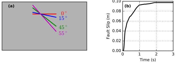
An 11-km × 8-km 2D homogenous linear elastic soil domain is considered for this study (Figure 1(a)). The shear modulus of the soil is 1.7 GPa, Poisson’s ratio is 0.3 and density is 1700 kg/m3. The resulting shear wave and P-wave velocities are 1000 m/s and 1870.8 m/s, respectively. To accurately model propagation of waves with a maximum frequency of 10 Hz, the soil domain is meshed using 4-noded quadrilateral elements (QUAD4) with a uniform mesh size of 10 m, and the simulation time step is set to 0.01s. This element size and time step criteria satisfy the guidelines outlined in Coleman et al. (2016).
Four earthquake fault configurations with dip angles of 0o, 15o, 45o and 55o are considered in this study. These earthquake faults are simulated using a set of 501 point sources spread evenly along each fault line shown in Figure 1(a). Each point source is a double couple and the energy released by this double couple depends on the fault configuration (i.e., slip, rake and dip of the fault), average slip time history, area of fault rupture and the shear modulus of the soil around the fault (Aki and Richards (1992)). To simulate an ideal plane wave, a fault of infinite length is required. The finite fault considered in Figure 1(a) can only simulate an approximation to a plane wave as the waves travel radially outward from the two ends of the fault. To simulate this approximation to a plane shear wave that travels perpendicular to the fault line, all the point sources are given the same slip time history and slip direction, and they are activated at the same time instant. The direction of the slip is chosen such that the soil above the fault moves left along the fault and the soil below the fault moves to the right along the fault (left lateral). The slip time history chosen for this analysis (Figure 1(b)) is an extension on simulations performed by the Southern California Earthquake Center and it has its basis in dynamic rupture simulations (Shi and Day, 2013). Modeling the earthquake scenarios using these point sources ensures that the same amount of energy is released in each scenario as only the dip parameter changes from one scenario to another.
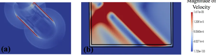
Snapshots of the waves generated from the four free-field earthquake rupture simulations are presented in Figure 2. Contours of the total velocity magnitude are plotted for each rupture scenario. The dark red regions in each image represent the maximum velocity magnitude of the wavefront of the inclined SV wave. As mentioned earlier, pure plane shear waves are generated only along the center section of the earthquake fault. Radial propagation of the seismic waves from the two ends of the faults can also be seen in these figures.
Figure 2: Snapshots of the free-field earthquake simulations with (a) 0o dip, (b) 15o dip, (c) 45o dip and (d) 55o dip showing the velocity magnitude for each simulation. The wavefront with the highest velocity
magnitude (red color) is the SV wavefront. The white line in each image is the earthquake fault.
a homogenous half space, the waves that are traveling in the downward fault-normal direction have to be absorbed when they arrive at the left, right or bottom boundaries of the soil domain. Lsymer dampers (Lsymer and Kuhlemeyer (1969)) are placed at these boundaries to absorb these outward traveling waves. Since Lysmer dampers only absorb completely waves incident at the boundary at a normal angle, Rayleigh damping with a small damping ratio of 0.05 % is also used throughout the soil domain to dampen any residual waves that are not completely absorbed by the Lsymer dampers.
The SV waves that travel in the upward fault-normal direction interact with the free surface. As mentioned earlier, the angle (measured from the vertical axis) at which these SV waves hit the free surface determines whether surface waves are generated or not. The angle of incidence of the SV wave in each of the four earthquake rupture scenarios is same as the dip angle of the fault in that scenario. For the first earthquake scenario with zero fault dip (Figure 2(a)), the SV wave is vertically incident on the free surface (incidence angle is 0o). The reflected wave in this scenario is just a downward traveling SV wave. In the second earthquake scenario with 15o fault dip, the SV wave is incident on the free surface at 15o and two body waves are reflected back from the free surface: (i) an SV wave with a reflected angle (also measured from the vertical axis) of 15o and (ii) a P (compressive) wave with a reflected angle of 29o. The reflected angle of the P wave is obtained using Snell’s law as shown below in Equation 1:
sin
i
V
S=
sin
r
V
P(1)
in which i and r are the incidence angle of the SV wave and the reflected angle of the P wave, respectively, and VS and VP are the S and P wave speeds, respectively. The wave fronts corresponding to these two reflected waves are visible near the free surface in Figure 2(b). As the incidence angle of the SV wave (i) increases, the reflected angle of the resulting P wave (r) also increases until it becomes 90o, i.e., the reflected P wave starts traveling parallel to the free surface. The incidence angle i for which r becomes 90o is called the critical incidence angle. For the soil considered in this study with a Poisson’s ratio of 0.3, the critical incidence angle is 32o. In the third and fourth earthquake scenarios, the incidence angle of the SV wave is 45o and 55o, respectively. Therefore, in Figures 2(c) and 2(d), there is no reflected P wave but instead a surface wave is generated.
VERIFICATION OF DOMAIN REDUCTION METHOD IN MASTODON
The Domain Reduction Method or DRM is a modular two-step finite-element methodology developed by Bielak et al. (2003) for solving complex earthquake engineering problems involving multiple physical scales. The traditional method to simulate the effect of four earthquake scenarios on five structures with different embedment depth is to run 20 simulations of the 11 km x 8 km soil-structure domain, each with one combination of earthquake fault dip and structure embedment depth. But the presence of a structure that is approximately 40 m wide and 14 m tall only influences the soil in the vicinity of the structure, i.e., a region with a radius of about 250 m (~ 6 times structure width) around the structure. With the use of DRM, the huge 11 km x 8 km soil + structure domain is divided into two parts: (i) the first simulation contains just the free-field linear elastic soil domain with the earthquake fault rupture as discussed in the previous section, and (ii) the results from this free-field simulation is transferred as input to a much smaller soil domain that is approximately 500 m x 250 m but contains additional features such as an embedded structure, nonlinear soil, etc. This reduces the computational effort significantly as the 11 km x 8 km soil domain has to be simulated only four times and additional complexities can be added to the smaller soil domain with ease and without increasing the computational cost of the overall simulation.
as the DRM element layer. This DRM element layer is located at the interface between the smaller soil domain used in part (ii) and the full free-field soil domain in part (i). These displacements are converted into a set of equivalent or effective forces that are then fed as input to the smaller soil domain at the same DRM element layer (black lines in Figure 3(b)).
Figure 3: (a) Free-field simulation of the earthquake fault rupture with 45o dip. The solid blue element layer near the free surface is the DRM element layer. (b) Smaller soil domain containing the exact properties of the bigger soil domain used to test DRM implementation in MASTODON. The black lines
here represent the DRM element layer.
The smaller soil domain (Figure 3(b)) considered for this test is 520 m wide and 280 m high. A 40 m soil layer is placed on the left, right and bottom of this soil domain and Lsymer dampers are placed at the ends of this extended soil domain to absorb any outward traveling waves. To verify the DRM method implementation, the smaller soil domain contains exactly the same features and soil properties as the bigger soil domain. For this particular case, if the DRM method is implemented correctly, the solution at every point inside the smaller soil domain should exactly match the free-field solution at the same location in the bigger soil domain. Also, the solution in the extended soil layer (located outside the DRM element layer in the smaller soil domain) should be zero as there are no additional features present in the smaller soil domain that can disrupt the dynamic equilibrium of the smaller soil domain + the DRM layer and only the scattered motion is calculated in the exterior region in the second step of the DRM. To obtain the total motion in this region, the reference motion in the initial step needs to be added to the scattered motion.
Figure 4: Horizontal (X) and vertical (Y) velocity time histories at the midpoint of the free-surface obtained from the bigger (solid red) and smaller (dashed black) soil domains.
ANALYSIS OF EMBEDDED NUCLEAR FACILITIES
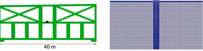
A generic nuclear facility structure (Figure 5(a)) is considered for this study. The width of the structure is 40 m and it is ~14 m tall. The structure is made of concrete with a Young’s modulus of 44 GPa, Poisson’s ratio of 0.2 and density of 2000 kg/m3. When the two footings at the lateral ends of the structure are modelled as fixed boundaries, the first two natural frequencies of the structures are at 8.2 Hz and 8.6 Hz and they correspond to the first modes in the horizontal and vertical directions, respectively. Rayleigh damping ratio is set to 4% for the structure.
Figure 5: (a) 40 m x 14 m generic nuclear facility model with a fixed base natural frequency of 8.2 and 8.6 Hz in the horizontal and vertical directions, respectively, and (b) smaller soil domain with the nuclear
facility embedded in the soil to 50 % of the structure’s height.
Five different embedment depths are considered for the structure – zero embedment or surface founded structure, 25%, 50%, 75% and fully embedded structure. The small soil+structure model for a structure embedment depth of 50% is shown in Figure 5(b). All the surfaces at which the structure and soil come in contact are tied together. The soil+structure model for the five different embedment depths are analysed using MASTODON under the equivalent force input obtained from the four free-field earthquake scenarios.
For each earthquake scenario and each embedment depth, the horizontal and vertical acceleration response spectra are obtained at the center of the second floor, indicated by the black rectangle in Figure 5(a). The horizontal (X) acceleration response spectra for all five structure-soil models and for each earthquake scenario are presented in the left column of Figure 6 (i.e., Figures 6 (a), (c), (e) and (g)). The corresponding vertical (Y) acceleration response spectra are presented in the right column of Figure 6. The colored curves in each subplot of Figure 6 correspond to the response spectra for the different embedment ratios.
In Figure 6, the response spectra for the surface-founded structures (black curves) peak around 7.25 Hz and 7.6 Hz in the X and Y directions, respectively, indicating that the interactions between the soil and structure decreases the fundamental natural frequency of the system from 8.2 Hz to 7.25 Hz in the X direction, and from 8.6 Hz to 7.6 Hz in the Y direction. It can also be seen that the response of the surface-founded structure is higher than the embedded structures in all the four earthquake scenarios. In fact, 25% embedment of the structure can reduce the response of the structure by half. However, further embedment of the structure does not result in significant additional reduction in the response of the structure, especially in the Y direction.
For the 0o dip earthquake fault scenario resulting in vertically propagating SV waves, the Y direction response is almost zero and the all the energy is in the X direction response as expected (Figures 6(a) and (b)). Therefore, the largest horizontal response of the structure is seen when the shear wave is vertically incident on the structure, and this horizontal response decreases with increase in dip angle. In the Y direction, the response of the structure increases with the dip angle up to a dip of 45o after which the response again drops for dip angle of 55o. But in all these cases the horizontal and vertical response of the surface founded structure is consistently higher than for the embedded structures.
From the preliminary results presented in this section, it can be seen that the embedment of the nuclear facility model significantly reduces the seismic response experienced by the facility.
CONCLUSIONS
The response of deeply embedded nuclear facilities to inclined earthquake waves is examined in this study using MASTODON finite element application. Four earthquake fault rupture scenarios with different dip angles, and 5 different structure embedment depths are considered for this study. Plane shear wave generation and propagation, and generation of surface waves for shear wave incidence angles (or fault dip angles) larger than 32o is demonstrated through free-field earthquake fault rupture simulations. Domain reduction method implementation in MASTODON is first verified and then used to simulate the response of embedded structures to earthquake input obtained from the free-field earthquake simulations. The different levels of embedment considered in this study vary from surface founded structure with no embedment to fully embedded structure.
The results from these preliminary analyses show that the response of the structure changes significantly with each earthquake scenario as the wave propagation direction changes the horizontal and vertical components of the ground motion. However, embedding the structure even to 25% of the structure’s height drastically reduces the response of the structure in all the earthquake scenarios considered. Further analyses with nonlinear soil material and non-tied contact between soil and structure are required to judge whether embedding the structure is always beneficial.
It is important to emphasize that the analysis conducted here considers that the structure and the soil respond linearly and that the structure and the soil move together at the common interfaces (i.e., no sliding or separations is allowed to occur). In actual situations, the soil present near the structure may deform nonlinearly due to the high strains generated due to soil-structure interaction. Also, the structure might slide at the soil interface or rock on the soil and these interactions may alter the final response of the structure. These effects need to be explored in detail before one can conclude that embedding the structure is always beneficial for all earthquake scenarios considered in this study.
REFERENCES
Achenbach, J.D. (1973). Wave propagation in elastic solids, North Holland.
Aki, K. and Richards, P. G. (2012). Quantitative Seismology, University Science Books.
ASCE/SEI 4-16 (2017). Seismic analysis of safety-related nuclear structures, American Society of Civil Engineers.
ASCE/SEI 43-05 (2005). Seismic design criteria for structures, systems, and components in nuclear facilities, American Society of Civil Engineers.
Bielak, J., Loukakis, K., Hisada, Y. and Yoshimura, C. (2003). “Domain Reduction Method for Three-Dimensional Earthquake Modeling in Localized Regions, Part I: Theory,” Bulletin of
Seismological Society of America, 93 (2), https://dx.doi.org/10.1785/0120010251.
Chen, W., Chatterjee, M., and Day, S.M. (1979). “Seismic response analysis for a deeply embedded nuclear power plant”, Proc. Structural Mechanics in Reactor Technology.
Coleman, J., Slaughter, A., Veeraraghavan, S., Bolisetti, C., Spears, R., Hoffman, W. and Kurt, E. (2017). “MASTODON theory manual”, Idaho National Laboratory.
Gaston, D., Hansen, G. and Newman, C. (2009). “MOOSE: A parallel computational framework for coupled systems for nonlinear equations,” in International Conference on Mathematics, Computational Methods, and Reactor Physics, Saratoga Springs, NY, 2009.
Hasegawa, M., Ichikawa, T., Nakai, S. and Watanabe, T (1987). “Nonlinear seismic response analysis of an embedded reactor building based on the substructure approach”, Nuclear Engineering and Design, 104(2), 175-186.
Longstreth, M., Appleford, A. and Tajirian, F (1991). “Soil structure interaction analysis of a deeply embedded reactor Silo”, Proc. International Conference on Recent Advances in Geotechnical Earthquake Engineering and Soil Dynamics, March 11-15, St. Louis, Missouri.
Lysmer, J. and Kuhlemeyer, R. L. (1969), “Finite Dynamic Model for Infinite Media,” Journal of the Engineering Mechanics Division, Proc. American Society of Civil Engineers, Vol. 95, EM4, pp. 859-876.
Masao, T., Takasaki, Y., Hirasawa, M. and Okajima, M. (1980). “Earthquake response of nuclear reactor building deeply embedded in soil”, Nuclear Engineering and Design, 58(3), 393-403.
Ostadan, F. (2006). "SASSI2000: A System for Analysis of Soil Structure Interaction - User's Manual," University of California, Berkeley, California
Shi, Z. and Day, S. M. (2013). “Rupture dynamics and ground motion from 3-D rough-fault simulations”,
Journal of Geophysical Research: Solid Earth, 118 (3) 1122-1141.
Wolf, J. P (1985). Dynamic soil-structure interaction, Prentice-Hall, Inc., Englewood Cliffs, NJ 07632. Xu, J., Miller, C., Costantino, C., Hofmayer, C., & Graves, H. (2006). Assessment of seismic analysis