University of Windsor University of Windsor
Scholarship at UWindsor
Scholarship at UWindsor
Electronic Theses and Dissertations Theses, Dissertations, and Major Papers
2012
Scene perception and motion planning through robotic vision
Scene perception and motion planning through robotic vision
Durga Rajan
University of Windsor
Follow this and additional works at: https://scholar.uwindsor.ca/etd
Recommended Citation Recommended Citation
Rajan, Durga, "Scene perception and motion planning through robotic vision" (2012). Electronic Theses and Dissertations. 136.
https://scholar.uwindsor.ca/etd/136
This online database contains the full-text of PhD dissertations and Masters’ theses of University of Windsor students from 1954 forward. These documents are made available for personal study and research purposes only, in accordance with the Canadian Copyright Act and the Creative Commons license—CC BY-NC-ND (Attribution, Non-Commercial, No Derivative Works). Under this license, works must always be attributed to the copyright holder (original author), cannot be used for any commercial purposes, and may not be altered. Any other use would require the permission of the copyright holder. Students may inquire about withdrawing their dissertation and/or thesis from this database. For additional inquiries, please contact the repository administrator via email
VISION
by
DURGA RAJAN
A Thesis
Submitted to the Faculty of Graduate Studies
through the Department of Electrical and Computer Engineering in Partial Fulfillment of the Requirements for
the Degree of Master of Master of Applied Science at the University of Windsor
Windsor, Ontario, Canada 2012
c
SCENE PERCEPTION AND MOTION PLANNING THROUGH ROBOTIC VISION
by
DURGA RAJAN
APPROVED BY:
Dr. Nader Zamani
Department of Mechanical, Automotive and Materials Engineering
Dr. Huapeng Wu
Department of Electrical and Computer Engineering
Dr. Xiang Chen, Advisor
Department of Electrical and Computer Engineering
Dr. Rashid Rashidzadeh, Chair of Defense
Department of Electrical and Computer Engineering
I hereby certify that I am the sole author of this thesis and that no part of this thesis has been published or submitted for publication.
I certify that, to the best of my knowledge, my thesis does not infringe upon anyone’s copyright nor violate any proprietary rights and that any ideas, techniques, quotations, or any other material from the work of other people included in my thesis, published or
oth-erwise, are fully acknowledged in accordance with the standard referencing practices. Fur-thermore, to the extent that I have included copyrighted material that surpasses the bounds of fair dealing within the meaning of the Canada Copyright Act, I certify that I have ob-tained a written permission from the copyright owner(s) to include such material(s) in my thesis and have included copies of such copyright clearances to my appendix.
I declare that this is a true copy of my thesis, including any final revisions, as approved by my thesis committee and the Graduate Studies office, and that this thesis has not been
submitted for a higher degree to any other University or Institution.
Abstract
The use of robotic vision is extensive in any field. This thesis aims to apply the theoretical concepts of the coverage strength model in order to achieve a task using robotic vision. The task mentioned is motion planning for the robotic arm such that it does not collide with an obstacle while performing its operation. This research can be applied to robots in an industrial work cell or an unmanned system. Hand in eye configuration is used to control
the robotic motion. Different levels of calibration are implemented, as a camera network is involved. An algorithm is used to implement the motion planning. This algorithm also involves the pose estimation of the objects used in the work cell. The work cell is modeled with a camera network and a robot. The calibration helps to visualize the position of the various entities of the work cell. The algorithm is applied to the physical experimental setup and results are recorded.
To my friends and family.
Acknowledgements
I would like to thank my advisor, Dr. Xiang Chen, for his guidance, encouragement and support throughout my masters studies. I would also like to extend my gratitude to Dr. Huapeng Wu and Dr. Nader Zamani for their valuable suggestions and comments.
I would like to take this opportunity to thank Dr. Maher Sid-Ahmed, Dr. Boubakeur Boufama and Dr. Ana Djuric for their guidance and help. I am grateful to my fellow
students, particularly Aaron Mavrinac and Jose Alarcon Herrera, who have helped me by providing useful comments at all stages of my masters degree.
I am grateful to the University of Windsor for the support provided in completing my masters degree. I would also like to thank the department technicians, Mr. Don Tersigni and Mr. Frank Cicchello, and the technical support center staff.
I thank my friends and family for their help and support.
Author’s Declaration of Originality iii
Abstract iv
Dedication v
Acknowledgements vi
List of Figures x
1 Introduction 1
1.1 Computer Vision and Robotic Vision . . . 2
1.1.1 Computer Vision . . . 2
1.1.2 Robotic Vision . . . 2
1.2 Autonomous camera equipped robot system . . . 3
1.3 Visual Sensor Network (VSN) . . . 3
1.4 Multi Sensor Robot System . . . 4
1.5 Literature Survey . . . 5
1.5.1 Robotic Vision in Industries . . . 5
1.5.2 Camera View Selection . . . 6
1.5.3 Purposive Sensing in Robotic Manipulators . . . 6
1.5.4 Obstacle Avoidance in an industrial robotic work cell . . . 7
1.6 Thesis . . . 8
1.6.1 Problem Statement . . . 8
1.6.2 Thesis Organization . . . 8
2 Theoretical Foundations 9 2.1 Geometry in Computer Vision . . . 9
CONTENTS viii
2.1.1 Transformations . . . 9
2.1.2 Pose Estimation . . . 10
2.1.3 Pose representations and composition . . . 11
2.1.3.1 Pose representations . . . 11
2.1.3.2 Pose Composition . . . 12
2.2 Camera Model and Calibration . . . 12
2.2.1 Pin Hole Camera Model . . . 12
2.2.2 Camera Calibration Theory . . . 16
2.2.3 Types of Camera Calibration . . . 18
2.3 Graph Theory . . . 20
2.3.1 Shortest Path Algorithm . . . 20
2.3.2 Camera Network Calibration using graph theory . . . 21
2.4 Coverage Strength Model . . . 22
2.4.1 Visual Stimulus Space . . . 23
2.4.2 Coverage Function . . . 23
2.4.3 Monocular Camera Coverage Model . . . 24
2.4.4 Discrete Model . . . 27
3 Scene Perception and Motion Planning Using Vision 29 3.1 General Solution . . . 29
3.1.1 Pose Type of the Robot . . . 29
3.1.1.1 Position Constant . . . 30
3.1.1.2 Joint Constant . . . 31
3.1.2 Robot’s motion planning to reach the target . . . 31
3.1.3 Estimation of the pose of the target and the obstacle . . . 32
3.1.4 Coverage Strength Data Computation . . . 33
3.2 Block Diagram of the System . . . 34
3.2.1 Functional Block Diagram . . . 34
3.2.2 Framework of the System . . . 35
3.3 Algorithm of the System . . . 36
4 Experiments and Analysis of Results 39 4.1 Preparatory Experiments . . . 39
4.1.2 Hand in Eye Calibration . . . 41
4.1.2.1 Pose Format Conversion for the robot . . . 42
4.1.3 Multi Camera Calibration . . . 44
4.2 Apparatus . . . 44
4.2.1 Experimental Setup . . . 46
4.2.2 Technical specifications of the robot and the camera . . . 47
4.2.2.1 Technical specifications of the robot . . . 47
4.2.2.2 Technical specifications of the camera and lens . . . 48
4.3 Experimental Procedure . . . 48
4.4 Results and Analysis . . . 50
4.4.1 Test 1 . . . 50
4.4.2 Test 2 . . . 52
5 Conclusions and Recommendations 66 5.1 Conclusions . . . 66
5.1.1 Overview . . . 66
5.1.2 Summary of Contributions . . . 67
5.2 Recommendations . . . 68
Bibliography 69
Appendix A Glossary of Terms 73
List of Figures
2.1 Perspective camera model (Image courtesy of [1]) . . . 13
2.2 Perspective projection of a point (Image courtesy of [1]) . . . 14
2.3 Calibration Pattern . . . 18
2.4 Chain of transformations for moving camera hand-eye calibration (Image courtesy of [2]) . . . 19
2.5 Multiple Camera Calibration . . . 22
2.6 Calibration Graph . . . 22
2.7 Axes and Angles ofD3 . . . 23
3.1 Tool Center Point pose of the robot (Image courtesy of [3]) . . . 30
3.2 Joint Axis (Image courtesy of [3]) . . . 31
3.3 Functional Block diagram of the system . . . 35
3.4 Framework of the system . . . 36
3.5 Simplified representation of the algorithm . . . 37
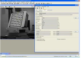
4.1 Calibration Assistant of Halcon machine vision library . . . 41
4.2 Image of the calibration target taken using the camera mounted on the robot during hand-eye calibration . . . 43
4.3 Pose Types available in Halcon . . . 43
4.4 Target mounted on the robot’s Tool tip . . . 45
4.5 Experimental setup. . . 46
4.6 The operation range at section X-X (Image courtesy of [4]) . . . 48
4.7 The work envelope for RV 1A . . . 49
4.8 Specifications of the CCD sensor (Image courtesy of [5]) . . . 50
4.9 Model File I . . . 55
4.10 Model File I contd.. . . 56
4.11 Preliminary test for the camera selection experiment . . . 57
4.12 Camera Selection results . . . 57
4.13 Obstacle Pose . . . 58
4.14 Target Pose . . . 58
4.15 MELFA IV BASIC program to communicate with the robot . . . 59
4.16 Target occluded by the obstacle in the vision platform . . . 60
4.17 Obstacle pose updated to the model . . . 61
4.18 Simultaneous Obstacle pose and target pose . . . 61
4.19 Robotic arm in movement towards the target . . . 62
4.20 Robotic arm moving away from the target . . . 63
4.21 Robot’s motion along the x-axis direction . . . 63
4.22 Robot’s motion along the y-axis direction . . . 64
4.23 Robot’s motion along the z-axis direction . . . 64
4.24 Target’s position along with the root mean square error . . . 65
Chapter 1
Introduction
Robotic manipulators have always been the major components of automated industries.
The design of an industrial robotic work cell is a complex issue and it is highly dependent on the application and the environment. A robot equipped with a camera works more effi-ciently and prevents the damages that could occur in an industrial setup that has no vision component for the robot. A camera network, also known as the vision sensor network, is always considered an essential element in a robotic work cell design. The use of visual information to control a robot has been used extensively in many sectors for various appli-cations. The vision sensor network in a robotic work cell helps to monitor the work cell
continuously. It leads to perceiving the entire scene in a robotic work cell. A dynamic work cell can be effectively controlled only with the help of a vision sensor network. This thesis also deals with a work cell consisting of a calibrated camera network. It is also interesting to note that a dynamic entity might enter this robotic work cell at any given time. These dynamic entities can either denote the target of interest or an obstacle to the target. The target of interest will be grasped by the robot’s end effector or gripper. The network of cameras helps to locate these dynamic entities and differentiate whether they are the
tar-get or obstacle. The robotic manipulator has to adapt to the position data provided by the vision sensor. The coverage strength model [6, 7] is used to achieve the detection and discrimination between the target and obstacle. The validation of the coverage strength model is found in [8] and an application of the coverage strength is found in [9]. Section 2.4 explains the coverage strength model in detail.
1.1
Computer Vision and Robotic Vision
1.1.1 Computer Vision
Computer Vision is the combination of image processing, pattern recognition, and artificial intelligence technologies, which focus on the computer analysis of one or more images taken with a single or multiple sensors. The analysis recognizes and locates position and
orientation, and provides a sufficiently detailed symbolic description or recognition of those imaged objects deemed to be of interest in the 3D environment [10].
Computer vision involves acquiring, processing and analyzing images in order to make certain decisions based on the output of the analysis. Computer Vision can be defined by discussing its problems. The primary issue of computer vision is computing the 3D properties of the world scene from the images acquired. The 3D properties are the geo-metric and dynamic properties of the world scene. Computer vision is a huge field and it
is still growing with new inventions and development. Areas related to image processing, robotics, artificial intelligence and pattern recognition merge effectively with computer vi-sion. Many terms and tools associated with computer vision overlap with other fields or disciplines. For instance, image processing is quite different from computer vision as it deals mainly with image to image transformations. The overlapping occurs due to the fact that images needs to be to pre processed using image processing techniques before they are given as inputs to the computer vision algorithms [11]. Computer vision has widespread
applications and offers an array of research topics. This thesis work addresses research areas related to “active and purposive vision” and “pose estimation” with application in “surveillance and hand-eye robotics systems”.
1.1.2 Robotic Vision
The term Robot vision is used for systems that take the principles of animated attention, purposive perception, visual demonstration, compatible perception, biased learning, and feedback analysis [10]. Robot vision can be assumed as an animated vision through the use of attention control. Almost all 3D vision applications are to be treated by analyzing images at different viewing angles and distances. This idea of animated vision operates on mechanisms of selective attention called attention control. Environmental Information that is more relevant for the vision task needs to be extracted for processing. These data may be
CHAPTER 1. INTRODUCTION 3
Data acquired proves useful only when it instantaneously perceives the scene in reality. There should always be a close relationship between the physical data acquisition and the appearance of the actual situation. After acquisition, images are processed using their
geometrical parameters. Compatibility holds between the geometric shape (global) and gray value structure (local) of the image. The output signals of the imaging processes need to be converted into 2D or 3D features. This in turn is fed to the downstream robotic control (arms, wheels).
1.2
Autonomous camera equipped robot system
A robot is a mechanical system which can be programmed to do a specific task. It consists of an actuator, which is mobile, and a controller fed with software. The software within the controller helps to solve the inverse kinematics. A camera equipped robot system can be used for two purposes: a vision supported robot system or as a robot supported vision system. The camera equipped robot could have the hand in or the hand off configuration. An autonomous robot system must incorporate four important characteristics, they are: appropriate interpretation of the situation, corporeality, competence and emergence. An
autonomous camera equipped robot system does autonomous task solving, which helps in visual perception and action. The characteristics of an autonomous robot system can be obtained by animated attention, purposive perception, visual demonstration, compatible perception, biased learning, and feedback analysis [10]. All these characteristics are inter -related and evolve from one another.
1.3
Visual Sensor Network (VSN)
Visual sensor network plays a major role in computer vision and its related fields. Visual sensor networks aided by human monitoring, were famous in the field of surveillance and security for a quite a long time. The feedback obtained from a visual sensor network can be used to control various robotic manipulators. A visually controlled robot can easily emulate the skills of a human being. Computer Vision algorithms have helped to eliminate the
network. A vision sensor network can be described as a distributed smart camera network. There are two types of VSN, they are: Homogeneous and Heterogeneous VSN. De-pending upon the requirement we can select the type of VSN necessary. This research
work involves homogeneous VSN system. In homogeneous VSN the camera sensor nodes are of same type and of similar capabilities, and are connected to one or more base sta-tions. In heterogeneous VSN the camera sensors are of different types and capabilities [12]. A VSN requires higher bandwidth and energy to transmit data. VSNs are also used for environmental monitoring, surveillance applications and industrial control. There are options available to process the image data locally at the camera level, which will reduce the transferring of data through the network. Hence, this function leads to the development
of a VSN that consists of totally independent and intelligent system of distributed cameras. This system provides only highly relevant input to the processing system (base station). The deployment of a visual sensor network in a robot work cell increases the effectiveness of the robot. This type of robot can function like a human being for certain tasks in dif-ferent industries. This type of VSN has strict boundaries on the maximum allowable delay of data from the camera to the processing unit. Yet another challenging task in VSN is
object tracking, since it is computationally intensive and it involves real time processing of images. This can be improved by increasing the number of views of the system. Another important feature of VSN is location and orientation of camera, which is obtained by the camera calibration process. This process is widely used in this project to locate the object in a precise manner.
1.4
Multi Sensor Robot System
Robots need to operate in an environment that is filled with uncertainties. The uncertain-ties could be with the perception of the environment, manipulator motion or task planning. Robots can easily perceive their environment if the environment is already known, but the task becomes complicated when the environment is uncertain. If there is going to be any unexpected motion in the work cell, the robot then faces the issue of moving without hindrance. This thesis deals with one of the uncertainties that could occur in a robotic
CHAPTER 1. INTRODUCTION 5
unstructured environment. Hence, it is necessary to use multiple sensors in order to make the robot movement robust, even in an unstructured environment. Instead of depending on a data from one single source, combining the data from multiple sources helps to reduce
uncertainty in the final decision taken. The main objective of a multi sensor network is to combine all the information from the different sources into a consistent environment description.
Multi-sensor systems have gone through many developments in recent years. Single sensor systems can only provide partial information about the system. Hence, multi sensor systems play a major role. Robot systems must use more than one vision sensor in a dy-namic manner in order to make the multi sensor robot system intelligent and autonomous.
1.5
Literature Survey
This thesis focuses on the collision avoidance of industrial robots, when there are changes in the environment of the robot’s work envelope. An approach is being adopted in this project in order to prevent the robot colliding with obstacles. Obstacles are modeled such that they can be tracked continuously with the help of a camera network. This section
discusses about some of the previous research works done, related to this thesis work.
1.5.1 Robotic Vision in Industries
Robots work in an environment that is customized according to the needs and dimensions of the robot. In industries many subsystems closely work together to guarantee a collision
free environment. Sensor system is the most critical subsystem. By making use of sensory equipments like cameras, the robot senses the environment and locates the objects (static or dynamic) that are blocking the path of the robot. As discussed by Brecht et al. [13], a human-robot coexistence system incorporated with a camera network was already proposed in [14] in the early nineties. They use reference images for detecting human operators and other obstacles. Their approach was not optimal with regard to computation time and memory requirements. In 1999 Steinhaus et al. [15] developed a MEPHISTO system,
systems a 360 field of view needs to be incorporated in the robotic vision system . In [17], a robotic vision system is built in order to avoid dynamic objects using a 3D camera. This robotic vision system requires a robot, a sensor and a logical unit to perform its task.
On the hardware side, a controlling program running on a PC evaluates the workspace data provided by the 3D camera. Accordingly, commands will be transferred to the robot thereby controlling its movements. In [18], Winkler et al. investigated the approach of dynamic collision avoidance. This involves artificial potential fields, visual servoing and impedance control. The software needs to be common for both the static and moving objects.
1.5.2 Camera View Selection
In [19], Tessens et al. have discussed the view selection in a distributed smart camera network. The mode of operation and precision of the output depends on the deployment of the camera network. The major advantage of the network is the elimination of occlusion problems. A limited number of additional views are used to obtain the desired observation.
The usage of smart cameras with in built image processing and a communication system will help to reduce the bandwidth usage required for networking. In [20], Monari et al. have discussed the several algorithms used for camera selection in sensor networks. It has been stated that the main drawback in all methods of camera selection discussed is the need for a learning period. Learning period is defined as the correspondences between objects disappearing in one camera and reappearing in another. This research work uses a model called coverage strength model for view selection. The coverage strength model has been
used more widely for sensor planning in literature than for view selection, as discussed in [9]. View selection using the coverage strength model establishes the smoothness of the view sequence, in addition to the selection of the best view [9].
1.5.3 Purposive Sensing in Robotic Manipulators
CHAPTER 1. INTRODUCTION 7
use of robotic manipulators has demonstrated increased manufacturing productivity. This increase depends critically on the simplicity with which the robot manipulator can be re-configured or re-programmed to perform various tasks. Actively placing the camera to
guide the manipulator motion has become a key component of automatic robotic manipu-lator systems. The vision-guided approach achieves high precision in manipulation along with improved productivity. For the assembly or disassembly tasks, a long-term aim in robot programming is the automation of the complete process chain, from planning to ex-ecution. Positional uncertainties are also an important error that needs to be considered in robotic vision. In the case of a hand in eye system, various factors like resolution, depth of view and field of view are taken into consideration. Kececi et al.[22] used a mobile
camera along with a 6 DOF robot to monitor a disassembly process. The optimal view pose is found from a set of candidate pose estimates. An optimal view pose, which avoids collisions and occlusions is determined. Hence, the optimal view pose helps for sensor planning in the work done in [22]. As per the survey done in [21], most of the purposive sensing methods designed for robotic manipulators deal with sensor planning and optimal sensor placement.
1.5.4 Obstacle Avoidance in an industrial robotic work cell
In [18], Winkler et al. discuss collision avoidance in industrial robots. They use the con-cept of artificial potential or force fields. The field is generated from the charges on the obstacles. The robot path control is achieved using impedance control. Image processing using a USB camera helps to find the position of the dynamic obstacles. The robot work
cell is monitored using one USB camera and the obstacle is mounted on the end effector of another robot. The obstacle position is found using step edge detection and Hough trans-form; after the obstacle detection, the path planning is done using artificial potential fields. In [23], Gecks et al. present an industrial work cell that is supervised by a group of sta-tionary cameras in order to prevent collisions due to human beings or obstacles. Difference image method is used to decide the robot’s path. Their paper helps to achieve safe human
1.6
Thesis
1.6.1 Problem Statement
In this thesis, the concept of visual feedback is used for robot’s motion planning. Robots play a major role in every part of life. They might offer assistance in the home, function as an appliance, or work in an industrial environment. Dynamic obstacles can be found in
any kind of work cell of a robot. Obstacle detection plays an important role in a dynamic environment. In an industrial robot’s pick and place application there might be dynamic obstacles in addition to the object to be picked. The approach taken for this thesis can be compared to a pick and place application where the target objects are in continuous movement on a conveyer belt. The overall objective is to detect occlusion of the dynamic target object and to prevent collision of the robotic arm with the dynamic obstacle. The robot’s movement has to be changed in order to avoid the dynamic obstacles. Dynamic or
static obstacles can disrupt the operation of any robot. The robot has to find a way to deal with the occlusion of the target object caused by dynamic obstacles. Collision avoidance is an important aspect in an industrial robotic cell. Hence, it is necessary for the robot to perceive an obstacle in order to prevent collision. The robot must reach the target when there are no dynamic obstacles that would cause collision between the obstacle and robotic arm. Once occlusion is detected the robot must change the direction of its motion such that it does not collide with the obstacle. The objective is achieved using a camera network
equipped with coverage strength model.
1.6.2 Thesis Organization
The objective and the important terms related to this research work have been explained in the previous sections. The literature relevant to the thesis topic has been discussed in Section 1.5. The rest of the thesis is structured as stated in the following paragraph.
Chapter 2 explains the theoretical concepts related to computer vision that will be used in the remaining chapters for the implementation of the thesis objective. The primary
Chapter 2
Theoretical Foundations
2.1
Geometry in Computer Vision
Robots seek the help of computer vision to detect and perceive the 3D environment. Geom-etry plays a major role in understanding the 3D structure of the robot’s environment. The three main geometry types involved in computer vision are Euclidean, Affine and Projective Geometry.
2.1.1 Transformations
The transformations involved during the formation of an image are based on the Euclidean, Affine and Projective geometry properties. Euclidean transformation, also known as the rigid transformation, is invariant to angles and distances. It involves a translation and rota-tion. The Euclidean transformation of vectorxcan be represented as given below:
E[x] =Rx+T, whereRrepresents rotation matrix andT represent the translation vector
from origin.
Also, Ris orthogonal anddet(R) =1. In Affine geometry the ratios and parallel prop-erty are invariants. Affine geometry is the super set of Euclidean geometry. Projective geometry is the most suitable for optics since optics require a perspective transformation. When the human eye looks at a scene, objects in the distance appear smaller than objects close by, which is known as perspective. Projective geometry is the super set of affine geometry. Here the invariant is cross-ratio. Point Pof an n-dimensional projective space has(n+1)homogeneous coordinates. A projective transformation fromPn toPm can be given asP→W P, whereW is(m+1)×(n+1)matrix and it has[(m+1)×(n+1)]−1
parameters. W denotes the transformation matrix from n-dimensional to m-dimensional space.W is a square and non-singular matrix, iff the projective transformation is a homog-raphy. Whenm=nthe projective transformation is termed homography. Hence, in a three
dimensional projective space each point has 4 homogeneous coordinates andW has 16 en-tries. The projective basis of Pnhas a set of (n+2)points. In a 3D projective space any five points in space can form the projective basis if no four points among them are copla-nar. In Affine geometry, the transformation matrixW has only 12 parameters, whereas in Euclidean geometryW has 6 parameters, which constitute the rotation and translational components [1].
2.1.2 Pose Estimation
Pose estimation is vital for any vision related task. The external calibration of a camera is also a pose estimation technique as explained in Section 2.2.2. Pose can be defined as a transformation required to map an object from its own coordinate system into an agreement with the sensory data [24]. The main objective of pose estimation is to find the pose of an
object in the image with reference to a coordinate system. The term pose denotes six com-ponents: the three rotational and three translational components. Pose is the combination of the position (translation) and orientation (rotation) data. Pose estimation can deal with a single, stereo or even sequence of images. The pose estimation method differs according to the object whose pose is found out. Certain methods work for a particular class of objects. The pose consists of a rotational and translational transformation. The rotational transfor-mation can be expressed using different notations according to the order of the rotation and
various other factors that will be discussed in the following section. The methods for pose estimation can be classified into three categories, they are listed below [25]:
1) Geometrical method: If the geometry of the object is known, then the projected image of the object in the camera is a function of the object’s pose, as the camera is calibrated. This method requires extracting some control parameters from the image, such as the cor-ners or features in order to establish the correspondence between the 3D scene points of the
object and its 2D image points. This research work also uses this method in order to find the pose of the target and the obstacle. Planar targets are used and their geometrical details determine the pose.
CHAPTER 2. THEORETICAL FOUNDATIONS 11
3) Learning based method: This uses a set of images of the object in arbitrary poses that are fed as inputs to the system. This indicates the learning phase of the system. Once this phase is over, the system will find the pose of the object when an image of the object is
provided.
2.1.3 Pose representations and composition
2.1.3.1 Pose representations
The important representation types used for the rotation component are discussed in this section.
1) Matrix representation: A rotation matrix R in Euclideann-space is an nxn real or-thogonal matrix, whose transpose is its inverse, and whose determinant value (det(R)) is equal to 1. The rotation matrix is generated from the Euler angles(φ,θ,ψ)by multiplying
the matrices obtained by the rotation through the X, Y and Z axis respectively.
2) Axis-Angle representation: Axis-Angle representation is also known as the expo-nential coordinates of a rotation. It expresses a rotation using two values: a unit vector representing the direction of the axis and an angle representing the magnitude of rotation about the axis.
3) Quaternion representation: Rotation is expressed in terms of a four dimensional nor-malized vector. It is the extension of complex numbers.
4) Euler Angles: Euler Angle represents the rotation around the three major axes: the x-axis, the y-axis, and the z-axis. We can represent any pose by the “roll” around the x-axis along the plane, the“pitch” around the y-axis, which extends along the wings of the plane, and the “yaw” or “heading” around the z-axis as a vector (roll, pitch, and yaw). The order of rotation can vary.
In this thesis the Euler angle representation and the matrix representation in homoge-neous form are mostly used to represent the rotational component of the pose.
The 3D rotation around an axis can be represented in multiple ways. In this research pose estimation is implemented using Halcon machine vision libraries 1. The pose rep-resentation types available in Halcon are given by the following parameters: ‘Order of Rotation, ‘View of Transform’ and the ‘Order of Transform’ [26]. By using different val-ues for these parameters various pose representation types are available. Each combination
of these parameter values represents a pose type and is indicated by a code ranging between 0 and 13. Section 4.1.2.1 explains Halcon pose types in detail.
2.1.3.2 Pose Composition
The relative pose of an object F with respect to an object A can be represented as PFA. This also represents an Euclidean transformation from the coordinate system ofF to that ofA. Pose composition is denoted by the symbolin this thesis. In case of a homogeneous
matrix representation of a pose, determining the composition of two poses simply means multiplying the two matrices corresponding to the two poses. A simple pose composition can be represented as follows:
PFP=PFAPAP (2.1)
Equation 2.1 denotes that the composition of ‘the transformation from the coordinate
system ofFto thatA’ and ‘the transformation from the coordinate system ofAto that ofP’ leads to the computation of ‘the pose transformation from the coordinate system ofFto that ofP’. This implies that the pose of an object with respect to another object can be found using a chain of intermediate poses in between them as determined by pose composition.
2.2
Camera Model and Calibration
This section describes the camera model and also camera calibration theory. The camera model is based on the perspective model. The camera calibration equations are derived from the pin hole camera model. Camera calibration is a method used to find the internal and external parameters of the camera.
2.2.1 Pin Hole Camera Model
Pin hole camera model is the basis of all camera models. It is also known as the perspective camera model and is most commonly used to approximate a real camera model. This model helps to understand the process of image formation and also leads to the formation of the calibration matrix. An image can be defined as a 2D transformation of a 3D structure with the help of a vision sensor. There are three coordinate systems involved for the 2D image formation using the pin hole camera model. They are: the image coordinate system, scene
CHAPTER 2. THEORETICAL FOUNDATIONS 13
result of a three step process, which is listed below:
Step 1) A 3D Euclidean transformation from the scene frame to the camera reference frame; Step 2) A 3D to 2D transformation from the camera reference frame to the image coordinate
system using perspective projective transformation;
Step 3) A metric conversion for the image to be defined in terms of pixels, using 2D Affine transformation.
The above three steps can be explained in detail. The final output of the above mentioned three steps is a calibration matrix. The pin hole camera model is represented in Figure 2.1. In Figure 2.1 the origin, O, represents the center of projection, Ox and Oy are parallel to the image plane and Oz represents the optical axis. The camera is attached to the reference
frame whose center is O [1].
Figure 2.1: Perspective camera model (Image courtesy of [1])
Step 1) 3D Euclidean Transformation:
follows: X0 Y0 Z0 1 =
r11 r12 r13 tx
r21 r22 r23 ty
r31 r32 r33 tz
0 0 0 1
X Y Z 1 (2.2)
In Equation 2.2, P= (X,Y,Z) and P0 = (X0,Y0,Z0) ; Also, r11,r12... represent the
ro-tational components and tx,ty... represent the translational components required for the
Euclidean transformation from the scene frame to the camera frame.
Equation 2.2 can be represented asP0=EP, whereE is a 4×4 matrix representing the displacement matrix.
Step 2) 3D to 2D transformation:
Using the triangle similarity properties in Figure 2.2 we get the following set of equa-tions:
Figure 2.2: Perspective projection of a point (Image courtesy of [1])
x= (X f)/Z (2.3)
CHAPTER 2. THEORETICAL FOUNDATIONS 15
In the Equations 2.3 and 2.4, xandyrepresent the image plane coordinates and f rep-resents the focal length. Also, these equations represent the projective transformation from 3D to 2D space. Assuming that f=1 this transformation can be represented as shown in
Equation 2.5 x y 1 =λ
1 0 0 0
0 1 0 0
0 0 1 0
X Y Z 1 (2.5)
Equation 2.5 can be represented as p=λIP, whereIrepresents the perspective
projec-tion matrix andλrepresent the scale factor.
Combining step 1 and step 2 the perspective projection of pointPcan be represented as
p=λIEP
Step 3) 2D-2D Transformation:
This transformation takes care of the conversion of scene units to pixels. In other words, it is a unit conversion from metric to pixel coordinates. If(x,y,1) represents a point pin the image plane using scenic units, then(u,v,1)represents the same point, p, in the image plane using pixels. The transformation from scenic units to pixel is achieved by using the scaling factorsαuandαv. The equations are listed below:
u=αux (2.6)
αu= f ku (2.7)
v=αvy (2.8)
αv= f kv (2.9)
A, A=
αu 0 u0
0 αv v0
0 0 1
(2.10)
Hence(u,v,1)T =A(x,y,z)T
We obtained three matrices from the three steps explained above. Combining the ma-trices E, I and A, we obtain the final matrix that represents the complete scene to image
transformation. This matrix is represented as M. Matrix M represents a projective trans-formation from the 3D to 2D space. It is a 3×4 matrix. Therefore M=AIE. MatrixM
can be written as shown in Equation 2.11 by ignoring the details of the individual matrix components. M=
m11 m12 m13 m14
m21 m22 m23 m24
m31 m32 m33 m34
(2.11)
The prospective projection of a 3D point P= (X,Y,Z,1) to the pixel coordinates p= (u,v,1)is given by Equation 2.12, whereλis a non zero scale factor [1].
u v 1 =λ
m11 m12 m13 m14
m21 m22 m23 m24
m31 m32 m33 m34
X Y Z 1 (2.12)
The elements of the matrixMdenote the extrinsic and intrinsic parameters of the cam-era, which are found out using Equation 2.12. This procedure is known as camera calibra-tion and it is explained in detail in Seccalibra-tion 2.2.2.
2.2.2 Camera Calibration Theory
CHAPTER 2. THEORETICAL FOUNDATIONS 17
The internal parameters of the camera determine certain properties of the camera, such as the focal length, image center, distortion coefficient, etc. As explained in the previous sec-tion the 3D point P must undergo a three step transformation in order to be transformed
into a 2D point in the image reference frame. Camera calibration involves a process that estimates the projection matrixM. The elements of the matrix,M, give the internal and the external parameters of the camera [1]. ‘Step 1) 3D Euclidean Transformation’ explained in Section 2.2.1 leads to the formation of the matrix E, which consists of 6 extrinsic pa-rameters of the camera. Also, ‘step 3) 2D-2D Transformation’ explained in Section 2.2.1 finds the four internal parameters of the camera according to the pin hole camera model. The estimation of matrix M starts with the process of adding two constraints to it, due
to the fact that M is defined up to a scale factor. The two constraints are m34=1 and
m312+m322+m332=1 . Note that the first constraint does not hold true iftz=0 and the second constraint is non-linear, which implies that the last row of the rotation matrix has a norm equal to 1.
Equation 2.12 leads to the formation of two projection equations. The estimation of ma-trixMis dependent on solving these two projection equations, which give the relationship
between the scenic points and corresponding pixels. The projection equations are listed below:
u= m11X+m12Y+m13Z+m14
m31X+m32Y+m33Z+m34 (2.13)
v= m21X+m22Y+m23Z+m24
m31X+m32Y+m33Z+m34 (2.14)
Estimation of the Equations 2.13 and 2.14 reveals that there are three sets of parameters
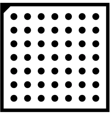
in which two are known quantities and one is unknown. They are: (u,v)denotes the 2D pixel coordinates that are known, (X,Y,Z)denotes the known 3D scenic coordinates and the 12 entries of matrixMdenotes the unknown quantities to be estimated. The 3D scenic points are known, as we use a calibration pattern similar to the one shown in Figure 2.3, whose geometric properties are known. The camera is set to the correct focus settings and the image of the calibration pattern is taken, from which the 2D points are extracted and matched with their corresponding 3D scenic points. These 2D and 3D points are used
assistant tool, Halcon. The experimental procedure related to camera calibration will be explained in Section 4.1.1.
Figure 2.3: Calibration Pattern
Note that the calibration theory to find the external parameters, which has been ex-plained in this section, holds true if the application involves only one camera. If there is a network of cameras involved, that is similar to that of this research work the procedure is different as explained in Section 2.3.2. In the case of multiple cameras, the geometric
re-lationship between the cameras needs to be established. The internal calibration procedure remains the same regardless of the number of cameras used. Also, this camera calibration theory is derived from the pin hole camera model, which uses perspective projection.
2.2.3 Types of Camera Calibration
This research work involves three different types of camera calibration. The experimental step by step procedure for each of these calibration techniques is explained in Section 4.1. The different calibration techniques used are as listed below:
CHAPTER 2. THEORETICAL FOUNDATIONS 19
dependent on the network. Internal parameters represent the properties of the camera. The theory behind internal calibration was explained in the Section 2.2.2.
2) Hand-Eye calibration: The term Hand-Eye evolved from the field of robotic vision
and it denotes the calibration of the camera with the robot. The robot can denote any system that helps to move objects like pan-tilt heads or multi-axis manipulators. There are two different kinds of hand-eye calibration based on the placement of the camera, which are moving camera hand-eye calibration (hand in eye calibration) and stationary camera hand-eye calibration (hand off eye calibration). The hand-eye calibration helps to find the relationship between the robot and the camera and the robot and the calibration target, respectively. In moving camera configuration the camera is mounted on the robot’s end
effector. In this configuration, the pose of the calibration target with respect to the base coordinate system of the robot, and the pose of the tool tip of the robot with respect to the camera coordinate system are determined [2]. The chain of homogeneous transformations that happen during this process is depicted in Figure 2.4.
Figure 2.4: Chain of transformations for moving camera hand-eye calibration (Image courtesy of [2])
In the stationary hand-eye calibration the camera is fixed in a position and does not move. This configuration helps to find the pose of the robot’s base with respect to the camera coordinate system and the pose of calibration target with respect to the robot’s tool coordinate system. This research work deals with the moving camera hand-eye calibration
and this steps involves only the camera that is mounted on the robot.
reference frame is vital information in order to perform any operation. The pose of each camera with respect to a common coordinate system is determined.
2.3
Graph Theory
The concepts of graph theory help to solve the issues in computer vision [27]. Some of the important terms of graph theory are discussed in this section. These terms will be used in the next section, which explains the calibration of a camera network. A graph is defined as a set of vertices connected using edges. The vertices are the nodes and the edges that denote the link between these nodes. In computer vision, the pixels or the interest points
can represent the vertices and the spatial relationships between them are denoted by the edges. If the vertices are represented by cameras, then the graph can be termed calibration graph, as explained in Section 2.3.2. These edges can be directed or undirected based on the application. Digraphs are the directed graphs in which the edges are given directions. In a digraph each edge is an ordered set of vertices. If there is an edge between two vertices,
vi andv j, they are termed to be adjacent, which would be denoted asvivv j. When the vertices of a path in the graph are distinct, except for the end vertices, the path is called a
cycle. Graph with no cycle in it is called acyclic. A tree is a connected acyclic undirected graph. A graph is termed bipartite if it can be partitioned into two parts, A and B, such that every edge of the graph connects the vertices in A to the vertices in B. Thus, matching in bipartite graph defines a one to one relation between the vertices in A and vertices in B. An undirected graph is connected if there is a path between any two vertices of the graph. A digraph is strongly connected if every pair of vertices has a directed path between them. A
connected graph has one connected component. In weighted graphs, a value is assigned to each edge. The shortest path between vertices is considered in terms of its length, where path length is given by the sum of all weights along the path.
2.3.1 Shortest Path Algorithm
The shortest path algorithm is used to find the shortest path distance between two vertices
CHAPTER 2. THEORETICAL FOUNDATIONS 21
algorithms make use of the fact that the a sub path within the shortest path is also the shortest. Dijkstra’s algorithm helps to find the shortest paths available from the source and assumes the weight of all the edges to be nonnegative. To compute the shortest path using
negative edge weight is nondeterministic polynomial time (NP) hard. The shortest path among all pairs of vertices can be found using the Dijkstra’s [28] algorithm recursively. The camera network calibration explained in Section 2.3.2 uses Dijkstra’s algorithm.
2.3.2 Camera Network Calibration using graph theory
The concepts of graph theory are used to perform the multi camera calibration. A graph
is said to be connected if a path exists from any point to any other point in the graph. The connected calibration graph is designed using the cameras and the target object at different orientations, as the vertices and edges denote the error of the associated poses. The calibration plate is used as the target object. The calibration target is placed at different orientations and the images are taken using the relevant cameras (the cameras in which the target appears in its Field of View). A subset of the camera network is formed for one
particular orientation of the target taken. A graph is constructed with the camera nodes and their associated target poses. One of the camera vertices is chosen to take the image of the calibration target whose absolute position is measured. This image is termed as the reference image or the reference target. Using Dijkstra’s algorithm [28], the shortest path from each camera vertex to the reference target is found. Once the shortest path is found, the pose composition is done to find the Pose of the source camera with respect to the reference target. The same procedure is repeated for all camera vertices, to find the
pose of each camera with respect to the reference target, along with a maximum aggregated estimation error.
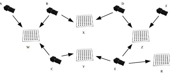
Figure 2.5 explains this calibration method with an example. One of the subsets of the cameras is represented by the camerasD,F andE with respect to the orientationZ of the calibration target. IfPAW denotes the pose of cameraAwith respect to the target orientation
W, then according to the Figure 2.5 we have the following poses:
PAW,PBW,PCW,PBX,PDX,PCY,PEY,PDZ,PFZ,PEZandPER
Figure 2.5: Multiple Camera Calibration
The shortest path will then beC,Y,E,R.
SoPCR =PCYPEY−1PER, where the symboldenotes pose composition.
This process is repeated for all camera vertices to find the shortest path that will finally
lead to the solutionPCjR, whereCjrepresents the camera.
Figure 2.6: Calibration Graph
2.4
Coverage Strength Model
The coverage strength model is a modeling approach applied to the sensor system, which is either monocular or multiple [6, 7, 9]. The various components of the coverage model
CHAPTER 2. THEORETICAL FOUNDATIONS 23
2.4.1 Visual Stimulus Space
The sensor coverage model requires a stimulus space to be defined in order to describe individual observable data [9]. A visual stimulus is localized to a point in three-dimensional
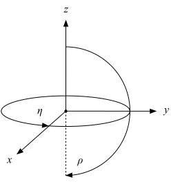
space, and also has a direction (normal to the surface on which the point lies; the view angle). This assertion is reflective of the fact that most, if not all, vision tasks can be reduced to operations on sets of point features [29, 30] and, furthermore, are or can trivially be made invariant to rotations about the principal axis, i.e. in the image plane. We therefore define adirectional spaceas the stimulus space for a system of vision sensors.
Definition 1 The directional spaceD3=R3×[0,π]×[0,2π)consists of three-dimensional
Euclidean space plus direction, with elements of the form(px,py,pz,pρ,pη).
We term p∈D3adirectional point. For convenience, we denote its spatial component ps= (px,py,pz)and its directional componentpd= (pρ,pη).
x
y z
ρ η
Figure 2.7: Axes and Angles ofD3
A rigid 3D pose P∈SE(3), represented by a rotation matrixR and translation vector
T, may be applied top∈D3. The spatial component is transformed as usual, i.e. P(p
s) =
Rps+T. The direction component is transformed as follows. Ifdis the unit vector in the direction ofpd, then
P(pd) =
arccos([Rd]z)
arctan 2([Rd]y,[Rd]x)
(2.15)
2.4.2 Coverage Function
Definition 2 A coverage function is a mapping C:D3 →[0,1], for which C(p), for any
p∈D3, is the strength of coverage atp.
Definition 3 The sethCi={p∈D3|C(p)>0}is the coverage hull of a coverage function C.
In order for the coverage function to offer a useful gauge of sensor system performance, it requires the context of a task, which minimally includes a definition of a coverage objec-tive overD3.
Definition 4 A relevance function is a mapping R:D3 →[0,1], for which R(p), for any p∈D3, is the coverage priority atp.
Given coverage and/or relevance functions Xi and Xj, we define their union and inter-section, respectively, as
Xi∪Xj(p) = max(Xi(p),Xj(p)) (2.16)
Xi∩Xj(p) = min(Xi(p),Xj(p)) (2.17)
for all p∈S. This, together with Definition 3, implies that hXi∪Xji=hXii ∪ hXji and
hXi∩Xji=hXii ∩ hXji.
2.4.3 Monocular Camera Coverage Model
The main components of the coverage strength model as described by Mavrinac et al. [9] are: Visibility , Resolution, Focus, Direction and Occlusion. They are explained in this Sec-tion. In defining the components of the single-camera model, we use a bounding function
B[0,1](x) =min(max(x,0),1) to limit x to the range [0,1], which simplifies the
formula-tion. We also letp0=PE−1(p), wherePE :R3→R3is the external pose of the camera, and
the transformation is applied to pas shown in Section 2.4.1 (thus,p0 isp in the camera’s coordinate system).
Given a task parameter γindicating a margin in the image (in pixels) for full coverage,
the horizontal and vertical cross-sections of the visibility component,CV, are given by
CV h(p) =B[0,1]
1
γh
min
p0x
p0z+tanαl,tanαr− p0x p0z
CHAPTER 2. THEORETICAL FOUNDATIONS 25
CV v(p) =B[0,1]
1 γv min p0 y
p0z+tanαt,tanαb− p0y p0z
(2.19)
forγ>0, where αl andαr are the horizontal field of view angles, and αt andαb are the
vertical field of view angles, as given by
αl=2 arctan
ousu
2f (2.20)
αr=2 arctan
(w−ou)su
2f (2.21)
αt=2 arctanovsv
2f (2.22)
αb=2 arctan
(h−ov)sv
2f (2.23)
where f is the focal length,suandsvare the effective pixel dimensions in units of distance,
ouandovare the pixel coordinates of the principal point, andwandhare the image (sensor) width and height in pixels. The completeCV is then given by
CV(p) =
min(CV h(p),CV v(p)) if p0z>0,
0 otherwise.
(2.24)
Given task parameters Rxi(maximum ideal resolution), Rxa(maximum acceptable res-olution), Rni (minimum ideal resolution), and Rna (minimum acceptable resolution), the
resolution component,CR, is given by
CR(p) =B[01] min p0z−zR(Rxa) zR(Rxi)−zR(Rxa), zR
(Rna)−p0z zR(Rna)−zR(Rni)
(2.25)
forRxi>RxaandRni<Rna, where
zR(R) =Rmin
w
tanαl+tanαr
, h
tanαt+tanαb
(2.26)
Given task parameters ca and ci, indicating the maximum acceptable and maximum ideal blur circle diameters, respectively, the focus component,CF, is given by
CF(p) =B[0,1]
min
p0z−zn z/−zn
,zf−p 0 z
zf−z.
forca>ci, where (z/,z.)and(zn,zf)are the near and far limits of depth of field as given
by (2.28), substituting blur circle diametersciandca, respectively, forc.
z= A f zS
A f±c(zS−f) (2.28)
In the preceding equation, A is the effective aperture diameter and zS is the subject distance. For many tasks, it is sensible forcito equal the physical pixel size, yielding the depth of field for perfect focus.
The direction (angle of view) component,CD, is given by
CD(p) =B[0,1]
cos(Λ(p0))−cosζa
cosζi−cosζa
(2.29)
whereζi,ζa∈[0,π/2]are task parameters indicating the ideal and maximum view angles,
respectively, andΛ(p)is the angle of view relative to the ray from the camera’s principal
point, which can be calculated as
Λ(p) =cos−1
sinpρcospη,sinpρsinpη,cospηT·ps
. (2.30)
Given a scene model S consisting of a set of triangles (which represent opaque faces of polyhedral objects in the scene), the point ps is occluded iff the point of intersection
between the line segment from ps to the camera’s principal point and any triangle inS2
exists, is unique, and is notps.
If V :R3 → {0,1} is a bivalent indicator function such that Vi(ps) =1 iff ps is not
occluded from camerai’s viewpoint, then the full coverage function is defined by
Ci(p) =CVi (p)CiR(p)CFi (p)CiD(p)Vi(ps) (2.31)
for allp∈D3.
Precisely speaking, the coverage function notationCi(p)is shorthand forCi(p,Ii,Ei,T,S),
2This intersection may be computed efficiently per M¨oller and Trumbore [31], for example. Furthermore, triangles inSwhich do not
CHAPTER 2. THEORETICAL FOUNDATIONS 27
where
Ii= (f,su,sv,ou,ov,w,h,A,zS) Ei= (x,y,z,θ,φ,ψ)
T = (γ,Rxi,Rxa,Rni,Rna,ci,ca,ζi,ζa)
are the intrinsic, extrinsic, and task parameter vectors, andSis the scene model. Because not all tasks have requirements matching all the task parameters, the “default” permissive values for T areγ=0, Rxi=∞, Rxa=∞,Rni =0, Rna =0, ci=1.0, ca=∞, ζi= π2, and ζa= π2.
2.4.4 Discrete Model
Given any pointp∈D3whereC(p) =1,CV,CR,CF, andCDare monotonic nonincreasing
functions over any half-space of D3 induced by a hyperplane through p. Thus, in the absence of occlusions — that is, where S=0/, or less restrictively,V(ps) =1 for all ps
in the projection of hCi on R3 — hCi is a convex polytope. However, in general,V is
not as well-behaved, andhCiis merely star-convex with respect to the camera’s principal point. This complicates the computation of hCii ∩ hCji, since, as shown by Tiwary [33], intersection of non-convex polytopes is NP-hard.
An arbitrarily close approximation can be achieved in the discrete domain. A coverage functionC has a discrete counterpart denoted as ˙C, such that ˙C(p) =C(p)for allp∈D˙3,
where ˙D3 is a discrete subset ofD3. We denote the summation ∑p∈D˙3C(˙ p)as |C˙|. Then,
given ˙Ciand ˙Cj sampled over a common ˙D3, ˙Ci∩C˙j can be computed exhaustively.
A discrete relevance function ˙Ralso allows computation of a bounded coverage perfor-mance metric for any coverage functionCas
F(C,R) =˙ ∑p∈hR˙iC(p)
˙
R(p)
∑p∈hR˙iR(˙ p)
(2.32)
where, by definition,F(C,R)˙ ∈[0,1].
In our coverage model, ˙R is the product of a task’srelevance model, which is a set of points in R3 and/or directional points in D3, each with an associated relevance value in
[0,1].
criterion inC, which is frequently useful, rather than defining separate coverage functions. Forps∈R3, we redefine (2.31) as
Ci(ps) =CVi (ps)CiR(ps)CiF(ps)Vi(ps) (2.33)
Chapter 3
Scene Perception and Motion Planning
Using Vision
3.1
General Solution
The general solution section explains the procedure used to obtain the robot’s position in terms of its Joint angular positions using the pose given by the camera mounted on the robot’s end effector. It is necessary to understand the pose convention used by the robot and the various terms involved with the syntax of the robot’s pose. Hence, the Section 3.1.1 explains the syntax for pose and joint constants of the robot.
This section also explains the pose estimation and coverage value estimation based on pose data of the target and obstacle.
3.1.1 Pose Type of the Robot
The various pose type representations were discussed in Section 2.1.3. The robot expresses its pose in the coordinate system of its tool. Hence, its angular representation is in the form of Euler angles. The robot used for experimental purpose is Mitsubishi RV-1A. This is a 6 axis robot with six rotational joints. The most commonly used command to control the robot in this research work deals with two important constants. They are joint and position
constants. The position constant denotes robot’s pose. The robot’s pose represent the pose of TCP (tool center point) with respect to the origin of the robot. The robot’s pose always starts with the letter P when it is defined in MELFA IV BASIC. MELFA IV BASIC is a programming language used to control the robot and teach points for it to move. It helps to
move the end effector of the robot to the defined target positions. The MELFA IV BASIC file must end with an empty line. Similar to the pose constant the robot’s movement can also be defined by using joint constant that has the angle of rotation with respect to each
joint of the robot. The joint constant also starts with letter J. The syntax for both position and joint constants are explained in the below sections [3].
3.1.1.1 Position Constant
Figure 3.1: Tool Center Point pose of the robot (Image courtesy of [3])
The position constant cannot contain any variables. The syntax is : P = (X,Y,Z,A,B,C,LI,L2)(FL1,FL2)
where,
• X,Y and Z indicate the coordinate data of the tool tip. Coordinate data is the position of the TCP with respect to the robot’s base in mm (millimeter) units.
• A,B,C represent the posture data, which is the orientation of the robot’s tool tip. A, B, and C are the robot’s posture in the coordinate system of its hand’s leading end (or flange center), each indicating a angle of rotation on the X axis, Y axis, and Z axis of the world coordinate system.
• L1, L2 are the additional axis data and are expressed either in mm (millimeter) or radians.
• FL1 represents the posture data. It is a binary number of length 7 whose last three digits provide the posture details.
CHAPTER 3. SCENE PERCEPTION AND MOTION PLANNING USING VISION 31
If the structure Flags (FL1 and FL2) are omitted the default value of (7,0) is taken. The additional axis data is mostly given as 0.
The coordinate and posture data of the robot are indicated clearly in Figure 3.1
3.1.1.2 Joint Constant
The syntax for Joint constant is as follows: J = (J1,J2,J3,J4,J5,J6,J7,J8)
J7 and J8 axis indicate the additional axis. The robot axis data are expressed in degree. Variables cannot be defined within this joint constant.
The robot’s rotational joints are shown in Figure 3.2
Figure 3.2: Joint Axis (Image courtesy of [3])
3.1.2 Robot’s motion planning to reach the target
robot is designed to move in a predefined set of movements at which cameraAcan cover the field of movement of the target within the workspace of the robot. Some of the important specifications of the Mitsubishi RV 1A robot are:
Pose Reliability -±0.02 mm (millimeter). Arm Reachable radius - 418 mm (millimeter).
The arm reachable radius helps us to visualize the work envelope of the robot. The work envelope of the robot is discussed in Section 4.2.2.1 and is shown in Figure 4.7. A set of pose transformation and compositions are done in order to help the robotic arm to reach the target. The compositions are done using homogeneous transformation matrices. The series of pose compositions done are illustrated below:
(Posetool camA)(Posetarget camA)−1= (Posetool target) (3.1)
(Posetool base)−1(Posetool target) = (Posebase target) (3.2)
(Posebase target)−1= (Posetarget base) (3.3)
The Posetool camA is obtained from hand-eye moving camera calibration (please refer Section 4.1.2). ThePosetool base is obtained from the robot’s controller. This denotes the robot pose.
Finally, Posetarget base denotes the robot’s pose used for reaching the target. The pose conversion to the robot’s pose configuration should be done before transmitting the pose
value to the robot. This pose value is converted to the joint configuration using the robot controller.
3.1.3 Estimation of the pose of the target and the obstacle
The pose of the target and the obstacle is estimated using Halcon machine vision library
functions. The target has a standard calibration pattern, hence finding the pose of the target is based on extraction of the calibration marks. In this case the descriptor file of calibration pattern used is included. This file has details in relation to geometric properties of the calibration pattern such as length and breadth of the pattern, the diameter of circles in the pattern, distance between the circles in the pattern, etc. The calibration pattern resembles the pattern shown in Figure 2.3.
The pose of the obstacle is estimated by creating a model of it. The obstacle chosen is of
CHAPTER 3. SCENE PERCEPTION AND MOTION PLANNING USING VISION 33
model for it. An image of the obstacle is taken by placing it along the Z-direction of the camera. In other words, the obstacle is placed perpendicular to the camera. This image is taken after the internal calibration of the camera. This image is fed as a template to create
descriptor model [26]. The descriptor model could be created using any of these detector types: Lepetit, Harris or Harris binomial. This model will be used for planar calibrated matching. Once the model is created, the obstacle pose is found during the experiment by matching the descriptor model with that of image data. The internal parameters of the camera must be provided in order to succeed in the pose estimation of both the target as well as obstacle. A major advantage of this technique is that the pose estimation succeeds even when the object of interest is partially occluded by another object. Also, the model
of obstacle must be created by each of the camera in the network before the start of the experiments. Model creation of the obstacle is one of the preparatory experiments to be done.
Sample output for pose estimation:
3D POSE PARAMETERS: rotation and translation
Rotation angles [degree] : r 141.029208993504 55.1707694587515 112.75893817857
Translation vector (x y z [m]): t -0.396276077712865 0.143798039521594 0.206699754969463
3.1.4 Coverage Strength Data Computation
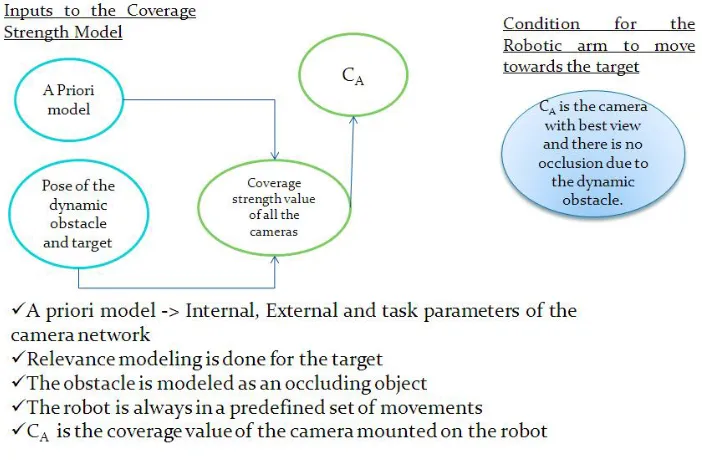
The theory behind the coverage strength model is described in detail in Section 2.4. The coverage strength model creates a model of the experimental setup with the help of the cal-ibration data. The data required to create the model is fed into a ‘.yaml’1file. For example,
the YAML file consists of the following data with regards to this research work:
1) The various task parameters and their optimal values are listed. The values of the task parameters vary according to the application. These default values of these task parameters are listed at the end of the Section 2.4.3.
2) The cameras used to build the network are listed along with their internal parameters and the external parameters with reference to a common frame as explained in the calibration
procedure of Section 4.1.
3) The scene data constitutes the next section of the YAML file. It has the pose details of all the elements that constitute the scene that includes the target and obstacle. The detection of occlusion is defined in Section 2.4.3.
4) The relevance data is provided in the form of geometric points that constitutes the bound-aries of the target. Refer the Definition 4 in Section 2.4.2.
The coverage strength value is calculated for each of the camera in the network based on
the data provided in the ‘.yaml’ file. The pose of the target and obstacle must be updated to the coverage strength model for it to provide the accurate coverage value of each camera. The coverage strength value of the target is dependent on the obstacle being out of target’s way. The ‘.yaml’ file that was used for the experiments is shown in the Figure 4.9 and 4.10 in Section 4.4.1.
3.2
Block Diagram of the System
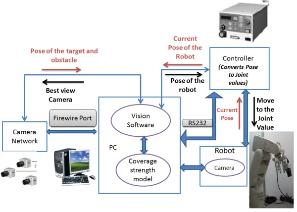
This section explains the important functional blocks and framework of the system.
3.2.1 Functional Block Diagram
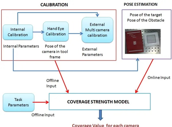
The functional block diagram as shown in Figure3.3, describes the important functional
blocks of the system, which helps to compute the coverage strength of each camera. The coverage strength computation plays a vital role in this system as it helps to decide on the camera to switch on and also to decide about the movement of the robot. The three main inputs provided are:
1) Calibration parameters 2) Task parameters
3) Pose estimates of the target and obstacle.
The calibration parameters (internal and external) and the task parameters are provided as a priori information to the coverage strength model. This priori information is recorded in the ‘.yaml’ even before the start of the experiments. More information about the task parameters can be found in the Section 2.4.3 and the calibration parameters are explained in detail in Section 4.1. The pose estimates of the target and obstacle are updated to the model online during the execution of the experiments and there is no priori information about it. The procedure used to obtain the pose of the target and obstacle is explained in
![Figure 2.1: Perspective camera model (Image courtesy of [1])](https://thumb-us.123doks.com/thumbv2/123dok_us/1437867.1176184/25.612.204.456.330.551/figure-perspective-camera-model-image-courtesy.webp)
![Figure 2.2: Perspective projection of a point (Image courtesy of [1])](https://thumb-us.123doks.com/thumbv2/123dok_us/1437867.1176184/26.612.187.457.367.597/figure-perspective-projection-point-image-courtesy.webp)
![Figure 3.2: Joint Axis (Image courtesy of [3])](https://thumb-us.123doks.com/thumbv2/123dok_us/1437867.1176184/43.612.224.391.315.502/figure-joint-axis-image-courtesy-of.webp)