Division V
EXPERIMENTAL IDENTIFICATION OF FLOW TURBULENCE
EXCITATIONS IN A FUEL BUNDLE TEST RIG: PART 1 -
EXPERIMENTS AND SOURCE IDENTIFICATION FROM LOW
AMPLITUDE ROD VIBRATIONS
José Antunes1, Valérie Biscay2, Philippe Piteau3, Xavier Delaune3, Alain Vivet2,
and Vincent Faucher4
1 Research engineer, IST-Centre for Nuclear Sciences and Technologies (C2TN), Estrada Nacional 10, 2695-066 Bobadela LRS, Portugal
2 Research engineer, Den-Département Technologie Nucléaire (DTN), STCP, LHC, CEA Cadarache, F-13115 Saint-Paul-lez-Durance, France
3 Research engineer, Den-Service d'études mécaniques et thermiques (SEMT), CEA, Université Paris-Saclay, F-91191, Gif-sur-Yvette, France
4 Project manager, Den-Département Technologie Nucléaire (DTN), DIR, CEA Cadarache, F-13115 Saint-Paul-lez-Durance, France
ABSTRACT
Flow-induced vibrations constitute an important factor in nuclear components degradation, particularly concerning the flow-excited tubular bundles of steam generators and fuel assemblages. In order to provide reliable predictive vibration computations, adequate flow excitation models are instrumental. In this paper we report preliminary experiments which emphasize the difficulties of source identification, as well as a method developed to tackle such challenge, for problematic, yet actual, vibration data. The experimental setup consists on a 5x5 bundle, assembled using four grids at uneven span lengths, subjected to axial flow. The experimental data consists on transverse vibration velocity responses measured at several locations along the rod, using a two-channel laser vibrometer. The vibration amplitudes were quite low, leading to noisy experimental data. Further difficulties included nonlinear effects at the supporting grids, as well as coupling between the orthogonal motion directions. As a result, the experimental data collected posed considerable difficulties for the source identification tasks. Here, an identification methodology is devised by constraining the investigated turbulence excitation to be of exponential spectral shape, enabling an optimal fit of the reduced spectrum parameters, amplitude and slope, to the experimental data. In addition, from the space distribution of the excitation, an estimate of the flow velocity profile is achieved. In a companion paper (Part 2 - Biscay et al., 2017) we present further measurements and computations which validate the source identification results obtained under such difficult conditions.
INTRODUCTION
The topic addressed in this paper is the identification of the spectral and spatial features of random flow turbulence excitations from vibratory responses. Previous efforts in this area, which are relevant to this work, include the pioneer work by Bolotin (1984) and the closely related theoretical and experimental study by Granger and Perotin (1999) and Perotin and Granger (1999), as well as later work by Park et al. (2009) and Hwang et al. (2009 and 2011). All these authors addressed the problem of source identification using modelling strategies anchored on a modal formulation of the structure dynamics. Based on a similar general approach but using new identification techniques, the present authors recently proposed a comprehensive framework for extracting the flow turbulence excitation features from vibratory responses, see Antunes et al. (2013a, 2013b and 2014). Their identification approach was tested on numerically simulated vibration data, for multi-supported bundles subjected to complex pattern flows such as those generated by turbulence grid spacers. Notice that system near-linearity and good signal-to-noise ration of the vibration data are assumptions required in all the above-mentioned investigations.
In Part 1 of the present work we present results from preliminary experiments under flow-excitation, performed at CEA-Cadarache, which somewhat defy such requirements, emphasizing the difficulties of source identification. The experimental setup consists on a 5x5 bundle with 1.3 m length and 10 mm rod diameter, assembled using four grids located such that the resulting spans are of uneven lengths. The test rig was subjected to axial flow with an average velocity of 5 m/s. The experimental data consists of transverse velocity responses measured at seven locations along the instrumented rod, using a two-channel laser vibrometer. Due to the considerable stiffness of the system, the measured RMS amplitudes were found to be quite low, in the range 1~3 microns, leading to noisy experimental data. Further difficulties of these experiments include nonlinear contact/friction effects at the supporting grids, as well as a strong coupling between the two orthogonal motion directions, while most measurement locations only allowed for a single measurement direction. As a result, the experimental data collected posed considerable difficulties for the source identification tasks.
Here, a pragmatic strategy is developed to tackle this challenge, for problematic, yet actual, vibration data. First, the modal response spectra and modeshape amplitudes are extracted from the physical response matrix, enabling identification of the system modal parameters from the modal responses. Then, the physical excitation spectra at various regions along the rod are identified and the reduced excitation spectrum and flow velocity profile are estimated. The system identification tasks closely follow the general framework proposed by Antunes et al. (2013a, 2013b and 2014). However, in order to deal with the present data, the excitation identification tasks implement here a less general but more robust strategy, based on a constrained optimization scheme, for extracting the crucial excitation features.
Actually, we have found that, for the identification of modal responses and modal parameters, the Second-Order Blind Identification (SOBI) technique could deal effectively with the experimental data. However, in order to proceed, our general identification methodology had to be modified by constraining the investigated excitation spectra to be of exponential shape, hence reducing the identification problem to an optimal fit of the reduced spectrum amplitude and slope. The identification results thus obtained appear realistic and, most importantly, in a companion paper (Part 2 - Biscay et al., 2017) we present further measurements and computations which validate the source identification results obtained.
FLOW-EXCITED VIBRATION EXPERIMENTS
Experimental setup
- flow rate between 1 and 200 m3.h-1, - pressure between 1 and 16 bars, - temperature between 50°C and 80°C.
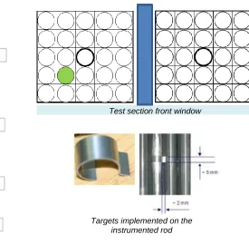
For the proposed measurements, the test section implements 2 reduced scale fuel assembly mock-ups (5x5 rod bundles with 1.3 m length and 10 mm rod diameter, one central guide tube and 4 grids, see Figure 1-a for the axial location of the grids) separated by a central wall, yielding two cavities with 67 mm x 67 mm section. One rod is instrumented for vibratory measures in one of the bundles (see Figure 1-b). The global conditions for the tests are given in Table 1, where two configurations are considered with different fluid velocities inside the bundles.
(a) Position of grids and targets for the instrumented rod
(b) Schematics of the test section with the location of the instrumented rod in the left tube bundle and view
of the targets for laser-doppler velocimetry
Figure 1. Test setup.
Table 1: Thermal-hydraulic test conditions.
Configuration 1
V1 = 5 m.s-1
Configuration 2
V2 = 7 m.s-1
Average flow rate per assembly 48.9 m3/h ± 2 % 68.5 m3/h ± 2 %
Pressure at the entry of the test section 6.0 ± 1 bar 7.5 ± 1 bar
Temperature at the entry of the test section 50 ± 2 °C 50 ± 2 °C
Laser vibrometers are used for contactless vibration measurements. Such devices are particularly suited for determining vibration velocity and displacement at fixed points. As detailed in Figure 2, the technology is based on the Doppler-effect, sensing the frequency shift of back scattered light from a moving surface. It is a relative velocity sensor consisting of a monochromatic light source (He-Ne laser λ=633 nm) and an interferometer. In our case, for more accessibility, we used laser fibber-optic vibrometers equipped with a mini-lens and a focusing system.
Test section front window
Figure 2. Contactless vibration measurements using a laser vibrometer.
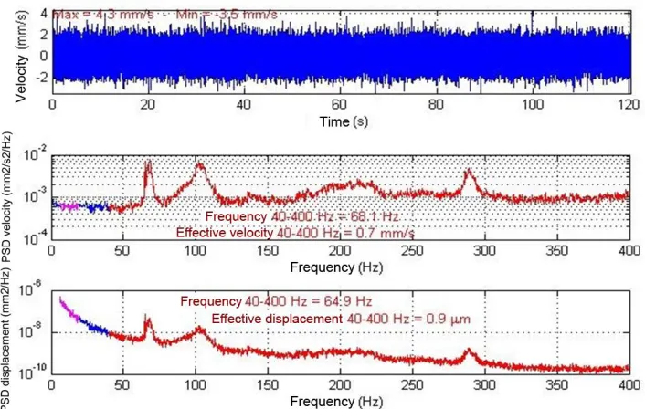
Experimental protocol: The selected rod is equipped with small targets with comparatively negligible mass (≈1g, see Figure 1-b). These targets are mounted on the rod at different elevations and orientations during the bundle handling. The vibration measurements on the rod, under axial flow rate (5 m/s), are performed using the two-channel laser vibrometer through the windows of the test section. The velocity of the rod is measured in the direction normal to the main test section window for Pt0 to Pt6 and also in the orthogonal direction for Pt4a, Pt5a and Pt6a (see Figure 1-a), using additional lateral windows. Data acquisition is performed at a sampling frequency of 1000 Hz during 600 s, for successive pairs of adjacent locations. The digitalized signals coming from the measurements carried out with the laser vibrometer were then processed through specifically developed Matlab software.
Figure 3. Example of vibratory measurements performed at Va=5 m/s.
Vibratory measurements
MODELLING TURBULENCE-EXCITED VIBRATIONS
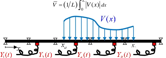
Figure 4 shows a generic system consisting on a beam-like structure with length L and diameter D subjected to a flow excitation with density
and velocity profile V x( )Vu x( ) , the normalieed flowprofile ( )u x being referred to the average velocity:
0
1 L ( )dx
V L
V x (1)Figure 4. Multi-supported tube subjected to a flow with generic velocity profile V x( ).
It can then be shown, see Axisa et al. (1990) and Antunes et al. (2012), that under linear conditions the cross-spectra of the random physical responses at generic locations xi and xj are given as:
1 1 , , 1, 2, ,
( ) YY( , , ) N N m( ) n( ) q qm n( )
ij i j n m i j i j R
S f S x x f x x S f
(2)
where m( )x and n( )x are the modeshapes and ( )
m n
q q
S f are the modal response cross-spectra, for
, 1, 2, ,
m n N. Formulations similar to (2) can be established to relate the physical and modal velocities,
as well as the physical and modal accelerations. The modal responses are formulated as:
*
1 2 1 2 1 2
0 0
( ) ( ) ( ) ( ) ( ) , ,
L L
n m n m FF
n m
q q
S f H f H f
x x S x x f dx dx (3)where 2
2 2
1( ) 4 2
n n fn n n
H f m f i f f , with the modal parameters mn , fn , n and n( )x of the
flow-subjected tube, while SFF
x x1, 2,f
is the cross-spectral function of the turbulence field, given as:
1/ 2
1 2 1 2
1, 2, ( , ) FF( , ) , ,
FF FF x f x f x x f
S x x f
(4)where
x x1, 2,f
is the space-coherence function of the turbulence eddies and the local excitationspectrum may, in dimensionless form, be approximated as:
2 2
21
( , ) ( ) ;
2 R R
FF FF
D fD
x f V u x D f f
V V
(5)
Then, we may write (3) as:
*
( ) n( ) m( ) ( )
n m F Fn m
q q
S f H f H f S f (6)
where the cross-spectra of modal forces:
2
( ) FF( ) nm( )
n m
F F
S f f L f (7)
depend on the following joint-acceptance and cross-acceptance correlation integrals:
1 22 2
1 2 1 2 1 2
0 0
( )
( )
( )
( ) ( )
,
,
nm n m
L L
dx dx
L
f
x
x
u x u x
x x
f
(8)Now, for near-homogeneous turbulence the space-coherence may be approximated by exponential functions, using Corcos (1964) model. For transverse (T) and axial (A) excitations, this leads to:
2 1
2 1 2 11, 2, exp 1, 2, exp exp
( ) ; ( ) ( ) 2
T A
c c c
x x x x x x
x x f x x f i
f f V f f
where ( )c f is a correlation length and ( )Vc f the convection velocity for the turbulence fluctuations.
Then, under the physically plausible hypothesis of small correlation length, ( ) /c f L 1, it can be shown from (5)-(9) that both cases can be approximated by a common formulation, see Axisa et al. (1990) and Antunes et al. (2012):
2 2 , , , , 2 1 2
( ) T A
T A EQR
T A T A
n m nm
F F
D fD
V D
V V
S f
C
(10)
with the "Equivalent Reference" transverse or axial flow turbulence excitation spectra, which are related to the corresponding local excitation spectra through (where LR is a postulated reference length):
1 2 1 2 ( / ) ( / ) ( / ) ( / ) ;
T T c T A A c A c A
EQR FF EQR FF
T T R A A R c A
f
fD V fD V fD V
fD fD fD fD
V V L V V L V fD V
(11)
and the simplified correlation integrals:
42 0
2 ( ) ( ) ( )
L
nm n m
C
x
x u x dx (12)When the simplified formulation (10)-(12) is adopted, both transverse and axial excitations may be dealt using a common theoretical framework, which is clearly advantageous from both the modelling and identification points of view.
IDENTIFICATION OF THE FLOW EXCITATION FEATURES
Identification strategy
A pragmatic strategy is developed in the following to tackle problematic experimental vibration data. The source identification is performed from a set of measured vibratory responses, following the four steps which will be now detailed: (1) The modal response spectra and modeshape amplitudes at the measurement locations are extracted through a blind decomposition of the physical response matrix; (2) The system modal parameters are identified from the modal responses using a simple SDOF identification algorithm; (3) Identification of the physical excitation spectra is performed using a constrained optimization scheme; (4) Finally, the reduced spectrum and flow velocity profile are estimated from the physical excitation spectra. Due to space reasons, only the results pertaining to flow velocity Va=5 m/s will be presented in the following.
(1) Identification of the modal responses
Given a number of modal auto-spectral response velocities Sˆq qn n( )f , n1, 2, ,N (where N is the
number of system modes significantly excited), formulation (2) shows how these can be directly related to a set of vibratory measurements Sij( )f SYY( ,x xi j, )f , ,i j1, 2, ,R. In matrix notation:
( )
qq( )
TYY
S
f
S
f
(13)where the modal matrix is
1 2 N
, with modal vectors n
n( )1 , , n( R)
T
x x
,
1, 2, ,
n N. On the other hand, for reasonably well separated modal frequencies, the modal response
velocities are nearly decoupled and equation (2) can be approximated as: 2
1
( ) , , 1, 2, ,
( ) ( )
n n
N
ij q q
n
x i j R
n i
S f S f
(14)
therefore, in practice, the matrix of modal responses
Sqq( )f
in (13) is diagonal. Then, as discussed bypriori information on the system modal properties, belongs to the class of Blind Source Separation (BSS) methods, a research area which is fast spreading into many fields, such as signal or image processing and system identification, for medical, engineering and science applications, see Cardoso (1998). The response equation (13) encapsulates an instantaneous mixture of the "source" vector of modal responses
Q t( )through modal matrix
, leading to the vector of physical measurements:
Y t( )
Q t( ) (15)Here, due to the nature of the excitation and the assumed linearity of the system, both
Q t( ) and
Y t( )will be Gaussian, therefore higher-order statistics do not apply to our problem. On the other hand, as mentioned before, matrix
Sqq( )f
is in practice near-diagonal, which implies second order independenceof the modal components of
Q t( ) . For such problem, the SOBI (Second Order Blind Identification)methods appear well suited, see Belouchrani et al. (1997). This technique exploits the correlation information contained in the measured response signals, being effective for separating sources with distinct power spectra, which is the case of modal responses for systems with non-degenerate modes. The SOBI method works in the time domain, using the correlation matrix of the physical responses, which is related to the spectral matrix through the Fourier transform [SYY( )]f F([RYY( )]) , hence:
( )
( )
TYY qq
R
R
(16)Because in practice only the cross-spectra between adjacent transducers could be measured, the original data matrix [SYY( )]f is tri-diagonal and all the remaining unknown cross-spectra Sij( )f were estimated
from the measured Si i(1)( )f using the iterative reconstruction technique developed by Antunes et al. (2016), based on a truncated SVD of the response matrix:
1 ˆ1 ˆ1
ˆ ( ) ˆ ( ) ( ) ( ) H
YY
S f f U f V f
(17)After performing the SOBI identification of the modal response spectra
( )
n n q q
S
f
and of the unscaled mixing matrix
ˆu
at the response locations, we estimated the corresponding continuous modeshapes ˆ ( )un x
along the tube by performing a spline interpolation through the values
{ }
ˆ
nu of each modal column of the mixing matrix
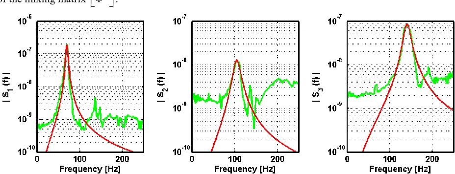
ˆu .Figure 5. Identified auto-spectra of the modal responses
( )
n n q q
S
f
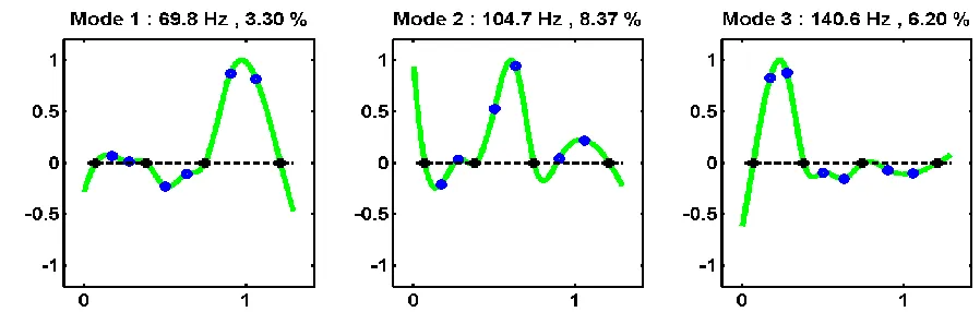
from the measured response matrix:Figure 6. Identified modeshapes ˆ ( )n x from the measured response matrix: Black = Support grids;
Blue = Measurement locations; Green = Interpolated modeshapes.
The results obtained are illustrated in Figures 5 and 6, for the first 3 identified modal responses and modeshapes of the rod, emphasieing the difficulties posed by the experimental data. In particular, interference from nonlinear and extraneous dynamics, as well as high noise levels, are responsible for a less-than-perfect separation of the modal responses. Even so, the experimentally identified modeshapes are in agreement with those obtained from a finite element model of the rod and supporting grids.
(2) Identification of the modal parameters
Before tackling the problem of identifying the modal excitations ( )
n n
F F
S f from the modal responses
( )
n n
q q
S f , one must identify the modal parameters mn, fn and
n from the modal responses. Actually, only the estimates of the modal masses mˆn depend on the quality of the estimates of the interpolatedmodeshapes ˆ ( )n x already obtained, shown in Figure 6. Indeed, the modal masses mˆn are estimated by assuming that the mass distribution (including the fluid added mass) m x0( ) is known a priori. Then:
0 0
2 2
0 0
ˆ ( ) ˆ ( ) ˆ ( )
L L
n n n
m
m x
x dxm
x dx (18)Once modal separation is achieved, it becomes easy to identify the other modal parameters by fitting to each modal response curve (either in the frequency-domain or in the time-domain) a SDOF identification algorithm. In the present study we decided to apply a modal identification technique in the frequency-domain, by minimieing the error:
2
1
1
2 2
2 2 2
2 2
ˆ
, , ( ) ( ) with ( ) 2
n n
f
n n n q q n n n n
f
FQ FQ
n n
C f S f C H f df H f f f f f f
(19)Table 2 shows the modal parameters thus identified, which again reflect the results obtained by a finite element model of the system. Also notice that the identified modal damping values are significant.
Table 2: Modal parameters identified after the SOBI modal extraction.
Mode 1 2 3
n
f (Hz) 69.8 104.7 140.6
n
(%) 3.3 8.4 6.2n
(3) Identification of the physical excitations
The excitation identification techniques proposed by Antunes et al. (2013, 2014) were found to be insufficiently robust to deal with the present difficult data. Therefore, we devised a constrained identification approach that, although lacking the generality of the mentioned efforts, proved robust enough for providing usable results. Following known results from a large corpus of experiments, we postulate that the investigated turbulence excitations will be of exponential spectral shape. For the case of a single slope, the reduced spectrum reads:
,
;
T A
EQR fR A fR fR fD V
(20)
with, if a two-slope spectrum is hypothesized:
, L R RC
L
H R RC
H f f A A f f A
(21)where the cut-off reduced frequency fRC lays at the junction between the low-frequency (L) and high-frequency (H) spectrum sides,
L HRC L H
f A A . With the constrained spectrum (20), the identification problem amounts to an optimal fit of the amplitude and slope spectral parameters to experimental data. Now, segmenting the rod length into PN space regions (N is the number of identified modes and modal responses), from equations (2), (6), (10), (12), (19) and (20) the following formulation is obtained:
1 1 1 1 1 1
2 2 2 2 2 2
2 2 2
1 1 1 2 1
1 2
2 2 2
1 2 2 1 2 2 2
2 1 2 1 ( ) ( ) ( ) ( ) ( ) ( ) ( ) ( ) ( ) ( ) ( ) ( ) ( ) ( ) ( ) ( )
N N N N N N
FQ FQ FQ
K K
FQ FQ FQ
K K
FQ F
K
N N
q q q q q q
q q q q q q
q q q q q q
H f H f H f
S f S f S f
S f S f S f H f H f H f
S f S f S f
H f H
2 2 22 2 2
1 2
11 11 11
1 1 1 2 1
2 2 2
1 2
2 1 2 2 2
22 22 22
2 2 2
1 2 1 2
( ) ( ) Q FQ N K P K P K
P P P P K
NN NN NN
f H f
C C C
f f f
f f f
C C C
f f f
C C C
(22)
where all the identified modes n1, 2, ,N are incorporated. The frequency dependent matrices are defined at all discretized frequencies fk f f1, 2, ,fK within the identified modal response peaks, which carry the relevant dynamical information. Also, beyond the already defined symbols, stands for the Hadamard term-by-term product of two matrices, the correlation integrals pertaining to the various modes and rod segments are:
max
min
2 2 1, 2, ,
1, 2, ,
2 ( ) ,
p p p nn n x x p P n N
C
x dx
(23)and the amplitude coefficients
p are given by:2 3 3
1, 2, ,
0.25
,
p
A D
V
p p P
(24)
where Vp V up( )x are the space-averaged physical flow velocities within the p1, 2, ,P rod
segments. Notice that (24) implies the physical non-negativity constraints: 1, 2, ,
0 ,
p p P
The unknowns in equation (22) are the P1 parameters
1, 2, , P;
in the case of a single-slope reduced excitation spectrum, or the 2P2 parameters
L1, H1, L2, H2, , LP, HP; L, H
in the case of a two-slope spectrum. Identification of these parameters is a nonlinear problem, which can be formulated through a constrained minimization of the error function:
2
2
, min n n(
)
( ) , ; subject to 0k
p
k k nn p k p
p q q n
f
S f H f C F f
(26)where we have expressed formulation (22) in compact notation. Several standard iterative schemes can be used effectively for such purpose.
(4) Identification of the reduced spectrum and velocity profile
After solving (26), one can recognize the difficulty of separating the spectral amplitude
A
from the flow velocity termsV
p encapsulated in the solution coefficients
p, see expression (24). This indeterminacywill be circumvented by referring the segment velocities
V
p to a reference mean velocity. As a practical approximation we will use the axial flow velocity in the test, so that:1
1 P
a p p
p L L
V V
(27)and such an assumption allows for the determination of
A
and theu
p
V
p/
V
a. In the present work, we have segmented the rod in PN3 regions. Because only three identified modes are used and their reduced modal frequencies encompass a somewhat limited frequency range, a single slope is assumed for the reduced excitation spectrum, as shown in Figure 7, which presents the equivalent reference turbulence excitation spectrum EQR
fR thus identified. On the other hand, the identified normalized effective velocity profile up is shown in Figure 8. A few comments on these plots are in order:1) Firstly, it appears that the identified reduced spectrum of the turbulence field generated by the axial flow and turbulence-generating grids is 2~3 orders of magnitude lower than the excitation spectrum of turbulence excitation from transverse flows, typified in Figure 7 by the reference excitation spectrum recommended by Axisa et al (1990).
2) This result is consistent with the usual practice when performing predictive vibration analysis of tube bundles subjected to axial flows. The typical excitation spectra used lay in the blue region of Figure 7. 3) Also notice that the single slope of the identified excitation spectrum in the present experiments seems compatible with the two-slope spectrum obtained by Axisa et al. (1990) for transverse flows.
4) Concerning the normalized velocity profile, one can notice that the flow velocity is maximal near the first grid, located at the flow entrance.
5) Finally notice that, from the theoretical rationale used for identification expressed in equations (11) and (12), both the identified excitation spectrum and flow velocity profile reflect turbulence excitation from the combined actions of axial and transverse flow components.
CONCLUSION
companion paper (Part 2 - Biscay et al., 2017) we present further measurements and computations which validate the source identification results obtained under such difficult conditions.
Figure 7. Identified equivalent reference turbulence excitation spectrum.
Figure 8. Identified normalized effective flow velocity profile.
ACKNOWLEDGEMENTS
The authors wish to thank AREVA and Electricité de France (EDF) for their support and contribution.
REFERENCES
Antunes, J., Delaune, X. and Piteau, P. (2011). "Time-Domain Modeling of the Random Vibrations of Tubes Subjected to Turbulence-Conveying Flows", ASME Pressure Vessel and Piping Conference (PVP-2011), Baltimore, USA.
Antunes, J., Borsoi, L., Piteau, P. and Delaune, X. (2012). "The Equivalent Spectrum Concept for Turbulence Conveying Excitations", 10th International Conference on Flow-Induced Vibration & Flow-Induced Noise (FIV-2012), Dublin, Ireland.
Antunes, J., Piteau, P., Delaune, X. and Borsoi, L. (2013a). "Spatio-Frequential Characterization of Turbulence Excitations Using Inverse Techniques: Part 1 - Extraction of the Modal Responses From the Vibratory Measurements", 22th International Conference on Structural Mechanics in Reactor Technology (SMiRT-22), S. Francisco, USA.
From the Modal Responses", 22th International Conference on Structural Mechanics in Reactor Technology (SMiRT-22), S. Francisco, USA.
Antunes, J., Borsoi. L., Delaune, X. and Piteau, P. (2014). "Identification of Random Excitation Fields from Vibratory Responses with Application to Multi-Supported Tubes Excited by Flow Turbulence",
ASME Journal of Pressure Vessel Technology, Vol. 68-69, pp. 431-448.
Antunes, J., Piteau, P., Delaune, X. and Borsoi. L. (2016). "Techniques for Estimating the Unknown Functions of Incomplete Experimental Spectral and Correlation Response Matrices", Mechanical Systems and Signal Processing, Vol. 136(5), Paper 051304-051304-13 PVT-13-1074.
Axisa, F., Antunes, J. and Villard, B. (1988). "Overview of Numerical Methods for Predicting Flow-Induced Vibration of Heat Exchanger Tube Bundles", ASME Journal of Pressure Vessel Technology, Vol. 110, pp. 6-14.
Axisa, F., Antunes and J., Villard, B. (1990). "Random Excitation of Heat-Exchanger Tubes by Cross-Flows", Journal of Fluids and Structures, Vol. 4, pp. 321-341.
Belouchrani, A.B., Karim, A.-M. and Cardoso, J.-F. (1997). "A Blind Source Separation Technique Using Second-Order Statistics", IEEE Transactions on Signal Processing, Vol. 45, pp. 434-444.
Biscay, V., Delaune, X., Piteau, P., Delafontaine, S., Antunes, J. and Faucher, V. (2017). "Experimental Identification of Flow Turbulence Excitations in a Fuel Bundle Test Rig: Part 2 - Flow Measurements and Vibration Computations for Validation", 24th International Conference on Structural Mechanics in Reactor Technology (SMiRT-24), Busan, South Korea.
Bolotin, V.V. (1984). "Random Vibration of Elastic Systems" (Chapter 8, pp. 409-416), Martinus Nijhoff, Hague, Netherland.
Cardoso, J.-F. (1998). "Blind Signal Separation: Statistical Principles", Proceedings of the IEEE, Vol. 86, pp. 2009-2025.
Chen, S.S. (1987). "Flow-Induced Vibration of Circular Cylindrical Structures", Springer-Verlag/Hemisphere Publishing Corporation, Washington, USA.
Corcos, G.M. (1964). "The Structure of the Turbulent Pressure Field in Boundary Layer Flow", Journal of Fluid Mechanics, Vol. 18, pp. 353-378.
Granger, S. and Perotin, L. (1999). "An Inverse Method for the Identification of a Distributed Random Excitation Acting on a Vibrating Structure. Part 1: Theory", Mechanical Systems and Signal Processing, Vol. 13, pp. 53-65.
Hwang, J.-S., Kareem, A. and Kim, W.-J. (2009). "Estimation of Modal Loads Using Structural Response",
Journal of Sound and Vibration, Vol. 32, pp. 522-539.
Hwang, J.-S., Kareem, A. and Kim, H. (2011). "Wind Load Identification Using Wind Tunnel Test Data by Inverse Analysis", Journal of Wind Engineering and Industrial Aerodynamics, Vol. 99, pp. 18-26.
Moussou, P., Bodel, C. and Benhamadouche, S. (2011). "CFD Estimation of the Unsteady Fluid Force Along a Fuel Rod Downstream a Mixing Grid". Paper PVP2011-57337, ASME Pressure Vessels & Piping Conference (PVP-2011), 17-21 July 2011, Baltimore, USA.
Park, N.-G., Rhee, H., Park, J.-K., Jeon, S.-Y. and Kim, H.-K. (2009). "Indirect Estimation Method of the Turbulence Induced Fluid Force Spectrum Acting on a Fuel Rod", Nuclear Engineering and Design, Vol. 239, pp. 1237-1245.
Perotin, L. and Granger, S. (1999). "An Inverse Method for the Identification of a Distributed Random Excitation Acting on a Vibrating Structure. Part 2: Flow Induced Vibration Application", Mechanical Systems and Signal Processing, Vol. 13, pp. 67-81.
Piteau, P., Delaune, X., Antunes, J. and Borsoi, L. (2012). "Experiments and Computations of a Loosely Supported Tube in a Rigid Bundle Subjected to Single-Phase Flow", Journal of Fluids and Structures, Vol. 28, pp. 56-71.