OUT-OF-CORE SIMPLIFICATION WITH APPEARANCE
PRESERVATION
FOR COMPUTER GAME APPLICATIONS
Project Leader Abdullah Bade
Researcher Assoc. Prof. Daut Daman
Mohd Shahrizal Sunar
Research Assistant Tan Kim Heok
RESEARCH MANAGEMENT CENTER UNIVERSITI TEKNOLOGI MALAYSIA
PRESERVATION
FOR COMPUTER GAME APPLICATIONS
PROJECT REPORT
Author Abdullah Bade
RESEARCH MANAGEMENT CENTER UNIVERSITI TEKNOLOGI MALAYSIA
Acknowledgement
Abstract
Abstrak
Table of Contents
CHAPTER TITLE PAGE
Acknowledgement i
Abstract ii
Abstrak iii
Table of Contents iv
1 INTRODUCTION 1
1.1 Introduction 1
1.2 Background Research 2
1.3 Motivations 5
1.4 Problem Statement 6
1.5 Purpose 6
1.6 Objectives 6
1.6 Research Scope 7
2 LITERATURE REVIEW 8
2.1 Introduction 8
2.2 Level of Detail Framework 9
2.2.1 Discrete Level of Detail 9
2.2.2 Continuous Level of Detail 10
2.2.3 View-Dependent Level of Detail 11
2.3 Level of Detail Management 11
2.4 Level of Detail Generation 15
2.4.1 Geometry Simplification 16
2.4.1.1 Vertex Clustering 16
2.4.1.2 Face Clustering 17
2.4.1.3 Vertex Removal 18
2.4.1.5 Vertex Pair Contraction 21
2.4.2 Topology Simplification 21
2.5 Metrics for Simplification and Quality Evaluation 23
2.5.1 Geometry-Based Metrics 23
2.5.1.1 Quadric Error Metrics 23
2.5.1.2 Vertex-Vertex vs Vertex-Plane vs Vertex-Surface vs
Surface-Surface Distance 24
2.5.2 Attribute Error Metrics 25
2.6 External Memory Algorithms 25
2.6.1 Computational Model 27
2.6.2 Batched Computations 27
2.6.2.1 External Merge Sort 27
2.6.2.2 Out-of-Core Pointer
Dereferencing 28
2.6.2.3 The Meta-Cell Technique 29
2.6.3 On-Line Computations 30
2.7 Out-of-Core Approaches 31
2.7.1 Spatial Clustering 32
2.7.2 Surface Segmentation 34
2.7.3 Streaming 36
2.7.4 Comparison 38
2.8 Analysis on Out-of-Core Approach 39
2.8.1 Advantages and Disadvantages 39
2.8.2 Comparison: In-core and Out-of-Core
Approach 39
2.8.3 Performance Comparison: Existing
Simplification Techniques 41
2.9 Appearance Attribute Preservation 46
2.10 Summary 48
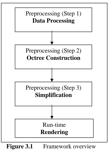
3 METHODOLOGY 51
3.2 Algorithm Overview 52
3.3 Data Processing 54
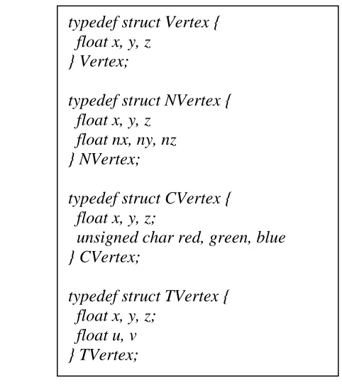
3.31 Data File Structure 55
3.4 Proposed Octree Construction 57
3.5 Proposed Out-of-Core Simplification 59
3.5.1 New Vertex Clustering 60
3.5.2 Generalized Quadric Error Metrics 61 3.5.2 Simplification on Internal Nodes 63
3.6 Run Time Rendering 64
3.7 Summary 65
4 IMPLEMENTATION 66
4.1 Introduction 66
4.2 Data Processing 67
4.2.1 Input Data Reading 67
4.2.2 Triangle Soup Mesh Generation 68 4.2.2.1 Calculation of Triangle’s
Dimension and Sorting Index 69 4.2.2.2 External Sorting on Sorting
Index 71
4.2.2.3 Dereferencing on Sorting Indices 72
4.3 Octree Construction 73
4.4 Out-of-Core Simplification 76
4.4.1 Simplification on Leaf Nodes 76 4.4.2 Simplification on Internal Nodes 76
4.5 Run Time Rendering 77
4.6 Summary 78
5 RESULTS AND DISCUSSIONS 79
5.1 Introduction 79
5.2 Octree Construction Analysis 80
Analysis 82 5.3.2 Relationships between Simplification and
Octree Construction 85
5.3.3 Surface-Preserving Simplification
Analysis 89
5.3.4 Comparison on Out-of-Core
Simplifications 91
5.4 Summary 93
6 CONCLUSIONS 94
6.1 Summary 94
6.2 Summary of Contributions 95
6.3 Future Works 97
REFERENCES 99
CHAPTER 1
INTRODUCTION
1.1 Introduction
A 3D interactive graphics application is an extremely computational
demanding paradigm, requiring the simulation and display of a virtual environment at interactive frame rates. It is significant in real time game environment. Even with the use of powerful graphics workstations, a moderately complex virtual
environment can involve a vast amount of computation, inducing a noticeable lag into the system. This lag can detrimentally affect the visual effect and may therefore severely compromise the diffusion of the quality of graphics application.
Therefore, a lot of techniques have been proposed to overcome the delay of the display. It includes motion prediction, fixed update rate, visibility culling, frameless rendering, Galilean antialiasing, level of detail, world subdivision or even employing parallelism. Researches have been done and recovered that the fixed update rates and level of detail technique are the only solutions which enable the application program balances the load of the system in real-time (Reddy, 1997). Of these solutions, concentration is focused on the notion of level of detail.
execution of the animation, object deemed to be less important is displayed with a low-resolution representation. Where as object of higher importance is displayed with higher level of triangle resolution.
The drastic growth in scanning technology and high realism computer simulation complexity has lead to the increase of dataset size. Only super computer or powerful graphics workstation are capable to handle these massive datasets. For this reason, problem of dealing with meshes that are apparently larger than the available main memory exists. Data, which has hundreds, million of polygons are impossible to fit in any available main memory in desktop personal computer. Because of this memory shortage, conventional simplification methods, which typically require reading and storing the entire model in main memory, cannot be used anymore. Hence, out-of-core approaches are gaining its attention widely.
As commonly known, graphics applications always desire high realism scene yet smooth scene rendering. Smooth rendering can be achieved by reducing the number of polygons to a suitable level of detail using the simplification technique. It saves milliseconds of execution time that help to improve performance. However, in order to obtain a nice simplified mesh, surface attributes other than geometry
information are essential to be preserved as well. Eye catching surface appearance certainly will increase the beauty of the scene effectively.
1.2 Background Research
Traditionally, polygonal models have been used in computer graphics
extensively. Till this moment, large variety of applications is using this fundamental primitive to represent three dimensional objects. Besides, many graphics hardware and software rendering systems support this data structure. In addition, all virtual environment systems employ polygon renderers as their graphics engine.
level of details has been used widely to reduce the complexity of the polygonal mesh using level of detail technique. In short, a process which takes an original polygon description of a three dimensional object and creates another such description, retaining the general shape and appearance of the original model, but containing fewer polygons.
Recent advances in scanning technology, simulation complexity and storage capacity have lead to an explosion in the availability and complexity of polygonal models, which often consist of millions of polygons. Because of the memory shortage in dealing with meshes that are significantly larger than available main memory, conventional methods, which typically require reading and storing the entire model in main memory during simplification process, cannot solve the dilemma anymore. Thus, out-of-core approaches are introduced consequently.
Out-of-core algorithms are also known as external algorithms or secondary memory algorithms. Out-of-core algorithms keep the bulk of the data on disk, and keep in main memory (or so called in-core) only the part of the data that’s being processed. Lindstrom (Lindstrom, 2000a) is the pioneer in out-of-core simplification field. He created a simplification method; called OoCS which is independent of input mesh size. However, the output size of the mesh must be smaller than the available main memory. Later on, other researchers carried out similar approaches.
Graphics applications, which demand high accuracy in simplification development is critical. It is essential to maintain the high quality and good frame rates at the same time. For example, medical visualization and terrain visualization is crucial in maintaining a good visual fidelity. Anyway, in many real time systems, the quality of data visualization has to be degraded in order to retain superior
rendering time. For instance, an excellent frame rate is vital in game environment without doubt. Thus, the quality of simplified model has to be sacrificed sometimes.
Rendering the large models at interactive frame rates is essential in many areas, includes entertainment, training, simulation and urban planning. Out-of-core techniques are required to display large models at interactive frame rates using low memory machines. Hence, it needs new solution or further improvement such as prefetching, geomorphing, appearance preservation, parallelization, visibility pre-computing, geometry caching, image-based rendering, and etc.
To avoid the last minute data fetching when needed, prefetching, visibility pre-computing and geometry caching are imperative. Although the changes from frame to frame are regularly small, however, they are occasionally large, so,
prefetching technique is needed. This technique predicts or speculates which part of the model are likely to become visible in the next few frames then prefetch them from disk ahead of time. Correa et al. (2002) showed that prefetching can be based on point visibility algorithms. Visibility can be pre-computed using from-region visibility or from-point visibility. Whilst geometry caching exploits the coherence between frames, thus keeping geometry cache in main memory and update the cache as the viewing parameters changes.
The geomorphing and surface preserving are potential in pleasant scene rendering. An unfortunate side effect of rendering with dynamic levels of detail is the sudden visual ‘pop’ that occurs when triangles are inserted or removed from the mesh. Geomorphing allows smooth transitions between the approximations
(Levenberg, 20002; Erikson, 2000; Hoppe, 1998a). In virtual environments or three dimensional game engines, the surface attributes play an important role to make the object looks attractive. Therefore, these surface attributes like colors and textures should be maintained after simplification process.
1.3 Motivations
Why do we care about visualization of large datasets? Due to the advances in scanning technology and complexity of computer simulation, the size of the datasets grows rapidly these years. The data is vital because it has application in many areas, such as computer design and engineering, visualization of medical data, modeling and simulation of weapons, exploration of oil and gas, virtual training and many more.
These massive data can only be rendered on high end computer system. If it is needed to run on personal computer, it may be an impossible mission, or even it can, the output is jagged or ungraceful. Therefore, to run it on expensive high end graphics machine, it is very cost ineffective and not user friendly. There is a need to display the data in low cost PC with high quality output.
1.4 Problem Statement
The datasets are getting enormous in size. However, even the well
implemented in-core methods no more able to simplify these massive datasets. This is mainly because in-core approach loads the whole full resolution mesh into main memory during simplification process. Besides, we cannot keep relying on high end graphics machine as it is expensive and not everyone has the chance to use it. Therefore, when the datasets bigger than the main memory, the datasets cannot be simplified.
Geometry aspects like vertex position always retained after simplification process whether in in-core simplification or out-of-core simplification. However, work in preserving the surface appearance, e.g. surface normal, curvature and color or even texture attributes in the original mesh is not common in out-of-core
simplification approach. The lost surface attributes will greatly reduce the realism of virtual environment.
1.5 Purpose
To render the massive datasets in 3D real-time environment and preserve its surface appearance during simplification process using commodity personal
computer.
1.6 Objectives
1. To develop an out-of-core simplification technique.
1.7 Research Scope
a) Only triangular polygonal mesh is considered, other data representation is not investigated here.
b) The simplification is for only static polygonal objects, dynamic object is not covered here.
c) Only vertex positions, normals, colors and texture coordinates are preserved after simplification process.
d) Application is run on commodity personal computer. Commodity in this content means low cost PC with not more than 2GB RAM and not any kind of SGI machine.
e) Graphics card of the PC is assumed capable in handling real time rendering.
f) Only simple level of detail management system is applied by using distance criterion.
g) Secondary memory used here is the hard disk, other secondary memory devices are not investigated its cons and pros.
h) The size of the datasets mustn’t larger than the size of secondary memory owned by the machine.
CHAPTER 2
LITERATURE REVIEW
2.1 Introduction
Mesh simplification reduces storage requirements and computational
complexity. For these reason, the scene rendering frame rate also becomes faster. In order to make the simplification suits into real time application, there are a few processes to go through. First, determine the level of detail framework to be used. Each LOD framework has its cons and pros. It is chosen based on application needs. Next, work on level of detail management to choose suitable or appropriate selection criteria. Then, to generate each level of detail for an object, simplification method is taken into account. For sure, metrics for simplification and quality evaluation is required as well.
The large datasets cannot be simplified using the ordinary in-core simplification methods as discussed before. It is inadequate. The large dataset simplification needs more mechanisms to make it run able in real time on low cost personal computer. First of all, the large dataset need to be loaded into system using external memory algorithm. Then, then data shall be organized into suitable
structure, which facilitate and accelerate the real time rendering. Last but not least, it has to be simplified using out-of-core simplification algorithm.
detail framework is discussed. Following it, Section 2.3 shows the level of detail management implemented so far. Then, researches that had been done in simplifying object are explained in Section 2.4. Next, the error metrics for simplification and evaluation are revealed in Section 2.5. Then, external memory management (Section 2.6) and out-of-core approaches (Section 2.7) are carried out. Later on, several comparisons carried out to differentiate all of the existing techniques (Section 2.8). Next, the appearance preservation is discussed in Section 2.9. Last but not least, this work is concluded in last section.
2.2 Level of Detail Framework
Currently, there are three different kinds of LOD framework, which are discrete LOD, continuous LOD and view-dependent LOD. Discrete LOD is the traditional approach, which is being used since 1976. Continuous LOD was developed in year 1996, while view-dependent LOD was created in the following year.
2.2.1 Discrete Level of Detail
Discrete level of detail creates several discrete versions of the object during a pre-process time. During run-time, it picks the most appropriate level of detail to represent the object according to some particular selection criteria. Many works select the appropriate level of detail using the distance aspect (Funkhouser and Sequin, 1993; Garland and Heckbert, 1997; Erikson et al., 2001). Since levels of detail are created offline at fixed resolutions, so it is called discrete level of detail or static polygonal simplification.
offline. It imposes very little overhead during run-time process. Secondly, it fits the modern graphics hardware well. It is easily to compile each level of detail into triangle strips, display list, vertex array and so on. Hence, it may accelerate the rendering process compared to unorganized list of polygons.
Even the implementation of discrete LOD is straightforward, popping artifacts may occur during level of detail switching. Besides, it is unsuitable for large datasets simplification if the whole simplified mesh is loaded during run-time without taking any viewing aspect into consideration.
2.2.2 Continuous Level of Detail
Continuous LOD is a departure from the traditional discrete approach. Discrete LOD creates individual levels of detail in a pre-process. Contrast to this, continuous LOD creates data structure, which enables desired level of detail can be extracted during run time.
2.2.3 View-Dependent Level of Detail
View-dependent LOD uses current view parameters to select best
representation for the current view. A single object may span several levels of detail. It is a selective refinement of continuous LOD. It shows nearby portions of object at higher resolution than distant portions (Hoppe, 1997; Luebke and Erikson, 1997; El-Sana and Varshney, 1999, Lindstrom, 2003b). Silhouette regions of an object may appear at a higher resolution than interior regions. View-dependent LOD can also take into account the user peripheral vision.
View-dependent LOD has better granularity than continuous LOD do. This is because it allocates polygons where they are most needed, within as well as among objects. For instance, one may consider a situation where only a part of object is near to viewer whilst the rest are not. If discrete LOD or continuous LOD is used, one may either use the high detail mesh or low detail mesh. It is rather unpractical as using the high detail mesh creates the unacceptable frame rates and the low detail mesh creates terrible fidelity.
The obvious disadvantage of view-dependent LOD is the increased loading time in choosing and extracting the appropriate LOD. If the system is run in real-time or CPU bound, this extra work will decrease the frame rate and subsequently induce lag artifacts.
2.3 Level of Detail Management
Level of detail management is an important process to choose the best level of detail for the object representation in different conditions. In deciding the most appropriate level of detail, different criteria have been developed to optimize the level of detail selection.
Basically a corresponding level of detail is applied based on the object’s distance to the user viewpoint. It may create visual ‘pop’ and does not maintain constant frame rate. The correct switching distance may vary with field of view, resolution and etc. However, it is extremely simple to understand and to implement.
A more sophisticated level of detail management is required to enhance the level of detail selection. Here, other implemented levels of detail selection
techniques are encapsulated as below:
a) Size
An object’s LOD is based upon its pixel size on the display device. It can overcome the weakness of distance selection criterion (Wernecke, 1993).
b) Eccentricity
An object’s LOD is based upon the degree to which it exists in the periphery of the display (Funkhouser and Sequin, 1993; Ohshima et al., 1996; Reddy, 1995; Watson et al., 1995). It is generally assumed that the user will be looking towards the centre of the display if suitable eye tracking system is absent. Thus, objects are degraded in relation to their displacement from this point.
c) Velocity
An object’s LOD is based upon its velocity relative to the user, e.g. its velocity across the display device or the user’s retina (Ohshima et al., 1996; Funkhouser and Sequin, 1993). Funkhouser and Sequin (1993) acknowledge that the objects moving quickly across the screen appear blurred, or can be seen only for only a short period of time, and hence the user may not be able to see them clearly.
images containing movement. This is probably point to slow moving object but not a fast moving object.
d) Fixed Frame Rate
Distinct from others, fixed frame rate concerns computational optimization rather than perceptual optimization. An object’s LOD is modulated in order to achieve a prescribed update rate. The refresh of screen must be in certain speed even sometimes the realism of scene has to be sacrificed.
Time-critical rendering ensures guaranteed frame rates even on scenes with very high complexity (Zach et al., 2002). This presented time-critical
rendering approach that combines discrete and continuous LOD selection and demonstrated its benefits in a terrain flyover application. The rendering process of every frame has to meet strict timing constraints to attain the best visual quality with the available rendering time.
e) Human Eyes Limitation
Resolution of element depends upon the depth of field focus of the user’s eyes. For example, objects out with the fusional area appear in lower detail. Highest sensitivity to spatial detail at fovea, other area is less sensitive. Another weakness of human eye is saccade. A saccade is a rapid reflex movement of the eye to fixate a target onto the fovea. Human do not appear to perceive detail during saccade.
There are two major influences on human visual attention: bottom-up and top-down processing. Bottom-up processing is the automatic direction of gaze to lively or colourful objects as determined by low-level vision. In contrast, top-down processing is consciously directed attention in the pursuit of predetermined goals or tasks. This technique demonstrated the principle of Inattentional Blindness (Cater, 2002), a major side effect of top-down
processing, where portions of the scene that unrelated to the specified task are unnoticed.
f) Environment Conditions
Slacken level of detail thresholds through the use of fog, haze, clouds, smoke, and etc. This is because these effects make the scene blur and hard to
perceive the actual detail.
g) Attention-Directed
This concept works out on where the user is likely to be looking at by using models of visual attention. Or, control where the user looks through the dramatic content of your scenes.
Visual attention-based technique allocates polygons to objects in a scene according their visual importance (Brown et al., 2003b). Every object is assigned an object importance value by considering the size, position, motion and luminance of the object. Then, a suitable level of detail will be taken for each object.
h) Shader LOD
2.4 Level of Detail Generation
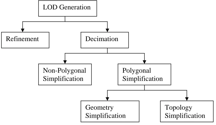
Automatic generation of various levels of detail is essential. Without this ability, multiresolution of meshes have to be generated manually. Such activity would be a tedious and laborious process. Hence, a variety of level of detail generation techniques has been proposed and generally known (Figure 2.1).
Figure 2.1 Level of detail generation classification
The most widespread methodologies in surface simplification are refinement and decimation. Refinement algorithm begins with an initial coarse approximation and adds details in each step. Essentially the opposition of refinement, decimation algorithm begins with the original surface and iteratively removes details at each step. Both refinement and decimation derive an approximation through a transformation from initial surface. Many algorithms have been developed in both approaches. However, decimation algorithm seems to have a more vital role in memory management.
Decimation simplification can either be polygonal simplification or non-polygonal simplification. Non-non-polygonal simplification includes parametric spline surface simplification, simplification of volumetric models and also image based simplification. For an example, Alliez and Schmitt (1999) minimize a volume using
LOD Generation
Refinement Decimation
Non-Polygonal Simplification
Polygonal Simplification
Geometry Simplification
the gradient-based optimization algorithm and finite-element interpolation model. Nooruddin and Turk (2003) also use voxel-based method with 3D morphological operators in their simplification. Practically, mostly all virtual environment systems employ polygon renderer as their graphics engine. Therefore, it is common to convert any other model types into polygonal surfaces before rendering. Hence, the polygonal model is ubiquitous. Pragmatically, the focus falls on polygonal model.
Polygon simplification can be categorized into geometry simplification and topology simplification. Geometric simplification reduces the number of geometric primitives such as vertices, edges, and triangles. Meanwhile, topology simplification deducts the number of holes, tunnels and cavities. Simplification that changes the geometry and topology of the original mesh is called aggressive simplification. Another idea from Erikson (1996) is that polygonal simplification can be separated into geometry removal (decimation), sampling and adaptive subdivision (refinement). Sampling is an algorithm that samples a model’s geometry and then attempts to
generate a simplified model that closely fits the sampled data.
2.4.1 Geometry Simplification
2.4.1.1 Vertex Clustering
The initial vertex clustering approach, proposed by Rossignac and Borrel (1993), is performed by building uniform grid of rectilinear cells, and then merging all the vertices within a cell, also can be call a cluster to a representative vertex for the cell. All the triangles and edges that stay completely in a cell are collapsed to a single point. Consequently, all these triangles and edges are discarded. Here by, the simplified mesh is generated.
“floating cell”. This floating cell algorithm dynamically picks the most important vertex as the center of a new cell, thus the quality is better.
Regularly, vertex clustering technique is fast and simple to implement. By recursively merging the clusters, the supercluster can be created. At the same time, it can be organized in a tree-like manner, allowing selective refinement of
view-dependent simplification.
2.4.1.2 Face Clustering
Face clustering is similar to vertex clustering as both also group a number of vertices into a cluster. However, face clustering is less popular than vertex clustering. The algorithm starts by partitioning the original faces into superface patches (Kalvin and Taylor, 1996). Then, the interior vertices in each cluster are removed, and the cluster boundaries are simplified. In a final phase, the resulting non-planar
superclusters are triangulated, thus creates a simplified model.
Garland (1999) creates multiple levels of detail for radiositized models by simplifying them in regions of near constant color. He uses the quadric error metric in simplifying the mesh’s dual graph.
2.4.1.3 Vertex Removal
Vertex removal method iteratively keeps taking away a vertex in each time, and its incident triangles are removed. In doing it, holes may be created and thus triangulation is needed. Perhaps this is one of the most natural approaches. The first vertex removal method was foremost introduced by Schroeder et al. (1992). They remove the vertex based on the distance between the vertex and the plane by fitting a plane to the vertices surrounding the vertex being considered for removal. Vertices in high curvature regions have the higher priority to be retained compared to the vertices in flatter regions during simplification process. This is because eliminating the vertex in high curvature regions induces more error.
Same like Schroeder et al. do, other works also make use of the error metrics. Simplification envelops (Cohen et al., 1996) algorithm removes the vertices
randomly as long as the simplified surface lies within the envelopes. It is ensuring the simplified mesh stays within a specified deviation from the original mesh. Klein et al. (1996) also coarsen the model using vertex removal technique with maximum error bounds guaranty.
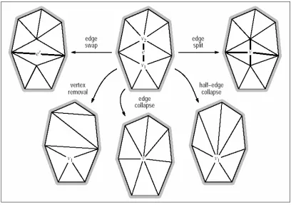
2.4.1.4 Edge Collapse
Edge collapse is the most popular simplification operator, invented by Hoppe et al. (1993). This operator collapses an edge to a single vertex, continuously
deleting the collapsed edge and its incident triangles. It is similar to vertex removal as it takes away a vertex at a time, yet, the choice of the vertex to be taken away is different. Also unlike vertex removal, no triangulation action is required because the resulting connectivity is uniquely defined
Progressive mesh (Hoppe, 1996) is the most famous work in existing edge collapse algorithms. A coarse mesh is keep adding details into it, explicitly, keep refining the mesh until a desired level of refined mesh is produced. It is done by performing the vertex split actions on the original mesh. This algorithm is wholly beneficial as the original coarser mesh can be obtained back by using the information used in vertex splitting process.
Edge collapse algorithm need to choose the order of edges to be collapse and also the optimal vertex to replace the discarded edge. Generally, these decisions are made by specifying an error metrics that depends on the positions of the substitute vertex. The sequence of the edges collapses usually is ordered from the cheapest to the most expensive action. In choosing the right replacement vertex, the lowest error metrics is used. Anyway, there are other factors may involve in these processes, including topological constraints, geometry constraints and handling of degenerate cases.
Haibin and Quiqi (2000) present a simple, fast and effective polygon reduction algorithm based on edge collapse by utilizing the “minimal cost” method to create multiresolution in real time 3D virtual environment development. Franc and Skala (2001) propose the parallel triangular mesh decimation using the edge contraction. The system is fast even sorting is not implemented. Its strength is proved according to the number of processors and the data size they used for testing.
Lindstrom and Turk (1998) create memoryless simplification using edge collapse, where geometric history in simplification is not retained. Then, the work was evaluated by Lindstrom and Turk (1999). Besides, memoryless polygonal simplification (Sourthen et al., 2001) applies vertex split operations in their level of detail generation.
Danovaro et al. (2002) compare two types of multiresolution representation: one is tetrahedron bisection (HT) and another one is based on vertex split (MT). Their work shows that HT can only deal with structured datasets whilst MT can work on unstructured and structured mesh. At the same time, based on their experiments, HT is more economic and the extracted mesh is lower in size.
An easier edge collapse method, commonly referred as half-edge collapse reduces an edge to one of its vertices. Hence, it generally produces in lower quality meshes than formal edge collapse since it allows no freedom in optimizing the mesh geometry. Anyway, as it allows the geometry to be fixed up-front, therefore it enables the polygon transferring and caching on the graphics card done efficiently. Besides, it is good in doing the view-dependent dynamic level of detail management. In addition, it is more concise and faster compared to edge collapse. This makes it suitable for progressive compression.
2.4.1.5 Vertex Pair Contraction
Vertex pair contraction is a variation of edge collapse that merges any pair of vertices from a virtual edge. There’s possibility to merge disconnected components of a model by allowing topologically disjoint vertices to be collapsed. Not every pair of vertices can be collapsed, basically the subsets of pairs, which are spatially close to each other, are considered. Different strategies have been introduced and the selection of the virtual edge is usually orthogonal to the simplification method itself, including Delaunay edges (1997) and static thresholding (1997).
The work of Erikson and Manocha (1999) is the most notable for its dynamic selection of virtual edges, which allows increasingly larger gaps between pieces of a model to be merged. According to the work of Garland and Heckbert (1997), the vertex pair contraction can be generalized to a single atomic merge of any number of vertices. Thus, vertex pair contraction is considered the primitive generation of the edge collapse and vertex clustering simplification method.
2.4.2 Topology Simplification
Topology refers to the connected polygonal mesh’s structure. Whilst, local topology of a primitive such as a vertex, edge or face is the connectivity of the primitive to their immediate neighborhood. If the local topology of a mesh is everywhere equivalent to a disc, then it is known as 2D manifold mesh.
Research on simplifying the topology of models with complex topological structure is gaining its attention. For large models with a large number of connected components and holes, such as mechanical part assemblies and large structures such as a building, it may need to merge the geometrically close pieces into larger
individual pieces to allow further simplification (Erikson, 2000).
close the holes in a mesh and hence the simplification is limited. Opposite to it, topology modifying algorithm aggregates separate components into assemblies, thus allows drastic simplification.
By default, the vertex pair contraction and vertex clustering are the
simplification operators that modify the topology of models. These operators are not purposely designed to do so, but it is a byproduct of the geometry coarsening process. Anyway, these operators may introduce non-manifold mesh after simplification takes place.
Schroeder (1997) keeps on coarsening the mesh using vertex splits when the half edge collapse is limited during the manifold preserving coarsening process. However, only limited topological simplification is allowed, for example, disconnected parts cannot be merged. The method proposed by El-Sana and Varshney (1997) is able to detect and remove small holes or bumps.
Nooruddin and Turk (2003) implement a new topology-altering
simplification, which able to handle holes, double walls and intersecting parts. Meanwhile, their work preserves the surface attributes and manifold of mesh at the same time. Liu et al. (2003) present a manifold-guaranteed out-of-core
simplification of large meshes with controlled topological type by utilizes a set of Hermite data as an intermediate model representation. The topological controls include manifoldness of the simplified meshes, toleration of non-manifold mesh data input, topological noise removal, topological type control and sharp features and boundary preservation.
2.5 Metrics for Simplification and Quality Evaluation
Geometric error metrics is a measurement of geometric deviation between two surfaces during simplification. Because of the simplified mesh is rarely identical to the original, therefore metrics is used to check how similar the two models are. For graphics applications that produce raster image or the visual quality of the model is highly important, thus the image metric is more suitable at this moment.
2.5.1 Geometry-Based Metrics
Besides evaluating the quality of the simplified mesh, metrics is determining the way of simplification works. This mathematical definition of metrics is
responsible in calculating the representative vertex and also determining the order of the coarsening operations. Anyway, each metrics has different ways in choosing its best manner for object simplification. On the other hand, the quality of the metrics is hardly to be evaluated in a precise way.
Typically simplification algorithms are using different kinds of metrics. Though, many of them are inspired by the well-known symmetric Hausdorff distance. This metric is defined using the Euclidean distance, which uses the shortest distance between a point and a set of points. In next sections, the well known metrics will be given away.
2.5.1.1 Quadric Error Metrics
Quadric error metrics (Garland and Heckbert, 1997) is based on weighted sums of squared distances. The distances are measured with respect to a collection of triangle planes associated with each vertex. This algorithm proceeds by iteratively merging pairs of vertices, which need not to be connected edge. Its major
contribution is a new way to represent error using a sequence of vertex merge operations.
Quadric error metrics efficiently represents the metrics by using matrix. Anyhow, it only supports wholly geometry simplification. Garland and Heckbert (1998) extends the metrics to more than four dimensions to support surface attributes preservation other than geometry information. The matrix’s dimension is based on how many attributes does a vertex own. It is particularly robust and fast. Besides, it produces good fidelity mesh even for drastic polygon reduction.
Quadric error metrics is fast, simple and guide simplification with minor storage costs. The visual fidelity is relatively high at the same time. In addition, it does not require manifold topology. That is, it allows drastic simplification as it lets holes to be closed and components to be merged.
2.5.1.2 Vertex-Vertex vs Vertex-Plane vs Vertex-Surface vs Surface-Surface Distance
2.5.2 Attribute Error Metrics
Quality evaluation can be done on image instead of model’s geometry. Image metrics have been adopted in a number of different graphics applications. Therefore, the quality of the simplified mesh can be measured by evaluating the difference before and after the simplification happens. Some image metrics are quite simple. Probably the traditional metrics for comparing images is the Lp pixel-wise norm. Nonetheless, recently there are quite a number of researches focus on humans’ psychology and vision to develop the computational models. In doing it, image processing and human visual perception is exploited.
Image processing techniques such as Fourier transform (Rushmeier et al., 1995) or wavelet transforms (Jacobs et al., 1995) can be used for this purpose. Besides, contrast sensitivity function also can be employed to guide the
simplification process. It measures contrast and spatial frequency of changes induces by operation.
Human visual perception is utilized by Watson et al. (2000) by conducting a survey on the human’s ability in identifying simplified models using different metrics. The durations of time spent to distinguish the different between the images for different metrics are analyzed. The results show that image metrics generally performed somewhat better than the geometry-based metrics used by Metro. Nevertheless, its robustness is uncertain.
2.6 External Memory Algorithms
other fundamental paradigms for external memory algorithms are introduced. Until now, researches on external memory are continuous and never end.
There are two fundamental external memory concepts used in visualization and graphics applications, including batch computation and on-line computation. Batch computation has no preprocessing process and the whole set of data is
processed. The way to make the data loadable is stream in the data in a few passes. Thus, only the portion of the data, which is smaller than the workstation’s memory, is filled at one time and processed. Whilst on-line computation conducts preprocess to organize the data into a more manageable data structure in advance. This
preprocess actually is a batch computation. Therefore, during runtime, only the needed portion of data is read into main memory by performing query on the well built data structure.
To accelerate the graphics rendering, geometry caching or prefetching techniques can be combined with the explained paradigms. It avoids the last minute data retrieval when the part of the data required to be displayed on screen. Else, it may slow down the rendering process as it needs to find the right portion of data from the data structure and then throw the required data to graphics card. Hence, if the part of the data, which is possible visible in the next frame is predicted, and put into cache first, consequently rendering will be speeded up.
2.6.1 Computational Model
Disk access is two times longer than main memory access (Aggarwal and Vitter, 1988). In order to optimize the disk accessing time, a large block of
contiguous data is loaded in one time. In handling large data sets, the size of input data (N) and the available main memory size (M) have to be found out.
Continuously, the size of the data item (B) has to be determined. It is the size of memory used for every pass of data reading or data processing.
The performance of external memory algorithms is based on the total of the I/O operations (Aggarwal and Vitter, 1988). This I/O complexity is calculated by dividing the size of input data by size of the data item (N/B). The data size of scanned data may be reaching a few hundreds million of triangles. For instance, LLNL isosurface datasets used in work of Correa (2003) is 473 million triangles.
2.6.2 Batched Computations
2.6.2.1 External Merge Sort
Sorting is the primary practice in large data management. This is because sorting eliminates the need of randomly searching on a wanted value lies in the large dataset. External merge sort is a k-way merge sort, that is, k is M/B. k is the
maximum number of disk block that can fit in main memory. The data is required to be loaded into main memory portion by portion in its contiguous place.
Basically, merging is made by comparing the values from different lists. For example, like in two-way merge sort, two lists of data will be merged into a single data list. These two lists are read from beginning, and then compare the first elements from both lists. Whichever smaller element is put into output list and the array pointer is incremented. Continue checking on the following elements in both lists until all data elements are completely sorted.
A memory insensitive technique (Lindstrom, 2000a; Lindstrom and Silva, 2001) practically use the external merge rsort written by Linderman (2000) It is a combination of radix and merge sort technique, which the keys are compare lexicographically.
The way of the sorted k sub-lists of the entire data (N) to be merged in good I/O complexity is important. These k sorted-lists are merged and output these sorted items to disk in units of blocks. When the previous buffer finished its process, then the next block of the corresponding sub-list is read into main memory to fill up the allocated buffer. This process is repeated until all k sub-lists are merged successfully.
2.6.2.2 Out-of-Core Pointer Dereferencing
Usually data used in visualization or graphics applications is in indexed format. The triangular indexed mesh has a list of vertex coordinates and a list of triangles indices pointing to its relevant vertex coordinates. This data format is compact and save memory space as every vertex value is only stored once.
Using indexed mesh needs full searching on the vertex list to find its
need several block by block data readings (B) from the entire input data (N). It would require (N) I/O’s in the worst case, which is extremely ineffective.
In order to make the massive data reading I/O efficient, thus the pointer dereferencing is used to replace the triangle indices by its corresponding vertices. Because of each triangle contains three vertices, so the pointer dereferencing also has three passes. In first pass, sort the first vertex using external merge sort technique. After all of the first vertices from triangle list are sorted, now the vertex list can be read in sequence. Keep replacing the vertex 1 with first vertex from vertex list, vertex 2 with second vertex from vertex list and so on. At that moment, all of the first triangle indices are filled with its equivalent vertices. In the second pass, sort the second vertices in the triangle list, and then dereference their equivalent vertices. Same works are acted upon the third vertices. Finally, triangle soup mesh is
generated with every triangle indices are filled with its corresponding vertices.
This technique is applied in Lindstrom’s (2000b) first out-of-core data simplification. Same with others’ opinion, his work also avoids random access by using triangle soup mesh instead of indexed mesh. This data representation is two to three times more space consuming, but typically increase simplification speed by a factor of 15-20 (Lindstrom, 2000b). This process has also been used in (Chiang and Silva, 1997; Chiang et al., 1998; El-Sana and Chiang, 2000; Lindstrom and Silva, 2001). These direct vertex information make the I/O complexity better.
2.6.2.3 The Meta-Cell Technique
isosurface extraction (Chiang et al., 1998; Chiang et al., 2001) and out-of-core volume rendering (Farias and Silva, 2001).
Basically the meta-cell technique divides the data into cells, which are equal in volume. Each meta-cell has own information and is normally loaded the whole from disk to main memory. The cell data is in indexed representation, called index cell set (ICS) by Chiang et al. (1998). This data representation contains a local vertex list and a local cell list, which point to the local vertex list. Hence, the vertex duplications are reduced compared to out-of-core pointer de-referencing technique. Only the vertices that fall into two different meta-cells are kept twice. Anyway, the more the meta-cells, the more the duplicated vertices it creates. However, it means each meta-cell is more refined and contains less information. Subsequently, the disk reading is faster. Therefore, there is always trade-off between query time and disk space.
The meta-cell technique has been extended for view-dependent simplification (El-Sana and Chiang, 2000). The meta-node tree is not only used in simplification but also accelerate the run time data query. At the same time, they also employ some additional features, such as prefetching, buffer management and also parallel
processing.
2.6.3 On-Line Computations
Tree based data structure significantly reduce the I/O complexity compared to direct data searching on the external memory mesh. Usually binary tree or even octree with branching factor two or eight can be used. Anyway, it still requires accessing a certain number of items in order to get the demanded item. Therefore, it is better to externalize the data structure to B-tree-like data structure. It can be done by increasing the branching factor for the internal node. Automatically, the tree’s height is decreased while the number of items in each node is increased. As a result, it can trim down the data searching time.
2.7 Out-of-Core Approaches
One of the reason why out-of-core simplification approaches exist is the majority of the previous methods for in-core simplification are ill-suited in out-of-core setting. The prevailing approach to in-out-of-core simplification is to iteratively perform a sequence of local mesh coarsening operations (Section 2.4.1) that locally simplify the mesh by removing a primitive geometry at one time. The order of operations performed relies on the error metrics they use, which discard a simplex according to their visual importance. In any case, manipulating the order of
coarsening operations from lowest error to highest error impose a certain number of memory and computational time.
In order to make the massive mesh able to be simplified, usually the mesh need to be partitioned until it is suitable to be simplified in available main memory. Therefore, it is common to group the mesh into clusters. Basically those triangles, whose vertices belong to three different clusters, are remained during the
simplification process. Ideally the partitioning is done to minimize the given error measurement and the representative vertex is chosen based on certain error metrics.
representation, where each triangle is represented independently as a triplet of vertex coordinated. The triangle soup can be generated by using the previously discussed external memory algorithms.
Varadhan and Manocha (2002) proposed an external memory algorithm for fast display of large and complex geometric environment. This algorithm uses a parallel approach to render the scene as well as fetch objects from the disk in a synchronous manner. Besides, novel prioritized prefetching technique that takes into account LOD switching and visibility-based events. Correa et al. (2002) also present an out-of-core preprocessing algorithm, which uses multiple threads to overlap rendering, visibility computation and disk operation. Besides, from-point
prefetching method is implemented. Crack prevention is introduced by Guthe et al. (2003) by appropriately shades the cut using fat borders in their hierarchical levels of details algorithm.
Borodin et al. (2003) also propose an out-of-core simplification with guaranteed error tolerance. The algorithm consisted three processes, includes memory insentive cutting, hierarchical simplification and memory insensitive stitching. Vertex contraction is their simplification operator as they claimed it produces better quality but slower computation time. Shaffer and Garland (2001) also propose an adaptive simplification of massive meshes, which can generate progressive transmission. It uses edge contraction in simplification process.
There are three distinct approaches to out-of-core simplification techniques: spatial clustering, surface segmentation and streaming (Lindstrom, 2003b). For each approach, uniform and adaptive partitioning will be distinguished.
2.7.1 Spatial Clustering
Determining cell containment performs vertex clustering. No topological constraints are considered.
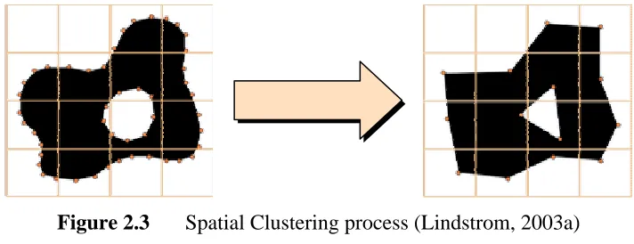
Spatial clustering’s main idea is to partition the space that the surface is embedded into simple convex 3D regions. Next, merge the vertices in the same cell. Because the mesh geometry is often specified in a Cartesian coordinate system, a rectilinear grid gives the most straightforward space partitioning. It is similar to vertex clustering algorithms (Section 2.4.1.1). Figure 2.3 illustrates the how the spatial clustering works.
Figure 2.3 Spatial Clustering process (Lindstrom, 2003a)
Uniform spatial clustering is simplest partitioning, which partitions the space into grid equally. It sparse the data structure represents occupied cells. By
For uneven triangles distributed mesh, where many triangles may fall in a region whilst the other part may have very little number of triangles, it is impractical to use the uniform clustering. It is because the uniform spatial clustering technique doesn’t adapt to surface features nicely. It does not imply well-shaped clusters. Besides, it may create many uneven or disconnected surface patches. On the other hand, the fixed-resolution limits the maximum simplification. To overcome these weaknesses, adaptive spatial clustering technique is proposed.
In adaptive clustering, the cell geometry is adapted to surface condition. For example, uses smaller cells in detailed regions. Garland and Shaffer(2002) present a BSP tree technique in space partitioning. Firstly, the quadrics on uniform grid are accumulated. Secondly, the PCA of primal/dual quadrics is used to a suitable space partitioning condition. In second pass, the mesh is reclustered. Fei et al. (2002) propose an adaptive sampling scheme, called the balanced retriangulation (BT). They use Garland’s quadric error matrix to analyze the global distribution of surface details. Based on this analysis, a local retriangulation achieves adaptive sampling by restoring detailed areas with cell split operation while further simplifying smooth areas with edge collapse operations.
2.7.2 Surface Segmentation
Fundamentally, spatial clustering partitions the space that the surface lies in. This method partitions the surface into patches so that they can be further processed independent in-core. Then, every patch is simplified to a desired level of detail using in-core simplification operator. For instance, one can simplify the triangles in the patch using the edge collapse. After simplification, the patches are stitched back.
As in spatial clustering, surface segmentation could be uniform by
Figure 2.4 Block-based simplification using uniform surface segmentation and edge collapse (Hoppe, 1998b)
Bernardini et al. (2002) propose a uniform surface segmentation algorithm with constraints that the boundary intact to allow future merging. It is quite easy to implement and have higher quality than spatial clustering simplification method. But, it is two times slower than spatial clustering method. Additionally, the output of the simplified mesh can’t span a few level of detail.
An adaptive surface segmentation algorithm is proposed, named OEMM (Cignoni et al., 2003c). It uses octree-based external memory mesh data structure. The grid is rectilinear and the data structure is unspecific that not only created for simplification purpose. It is similar to Bernardini et al. (2002), but the octree adapts in suitable resolution to match better surface detail, the edges can be collapsed across patch boundaries and the output is a progressive mesh.
Prince (2000) uses octree partitioning and edge collapse like OEMM do. He is able to create and view progressive mesh representation of large models. He uses octree partition, edge collapse simplification operator but need to frozen the path’s boundary. There is another adaptive surface segmentation method is by Choudhury and Watson (2002) whose propose a simplification in reserve. It is an enhancement of RSimp (Brodsky and Watson, 2000) to become VMRSimp. Brodsky and Watson use refinement based on vector quantization. Their work is generally believed faster as the refinement is take shorter time than simplification does. Anyway, it has poorer quality as refinement leads to lower quality result.
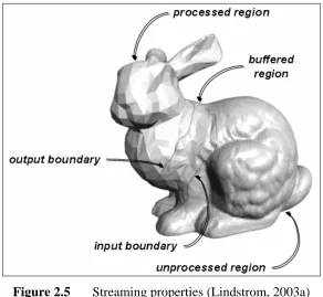
2.7.3 Streaming
Streaming treats a mesh as a sequenced stream of triangles. For each time, read a triangle, process it then write it in a single pass. Later on, in finite in-core stream buffer, indexed submesh is built up. For the triangles that loaded into buffer, in-core simplification is performed. In order to make sure buffer contains
sufficiently large and connected mesh patches, it requires coherent linear layout of mesh triangles.
Figure 2.5 Streaming properties (Lindstrom, 2003a)
A new approach in out-of-core mesh processing technique can be adapted to perform computation based on new processing sequence (Isenburg and Gumhold, 2003; Isenburg et al., 2003a) paradigm. Processing sequence for large mesh simplification (Isenburg et al., 2003b) represents a mesh as a particular interleaved ordering of indexed triangles and vertices. This representation allows streaming very large meshes through main memory while maintaining information about the
2.7.4 Comparison
The Table 2.1 shows the comparison between these out-of-core simplifications based on different attributes.
Table 2.1 Comparison between 3 types of out-of-core simplification Characteristics Spatial Clustering Surface
Segmentation
Streaming
Concept Cluster vertices
based on spatial proximity
Cluster vertices primary based on error
Cluster vertices based on spatial or error-based criteria Speed Fast (50-400K tps) Slow (1-10K tps) Fast and highly
parallelizable via pipelining
Quality Low High Governed by user
specific stream buffer
Suitable situation Time or space is at premium. Quality more important than speed, need progressive streaming, view-dependent rendering and preserve topology
Need to preserve connectivity, need high quality
Main drawback Low quality, topology not preserved
Slow Not clear how to
create
multiresolution meshes
2.8 Analysis on Out-of-Core Approach
2.8.1 Advantages and Disadvantages
Nowadays, models are well beyond most core memories can be handled. The sizes of these datasets rise drastically from range 107 to 109 faces. The out-of-core approaches apparently solved simplification problems on datasets, which are larger than main memory. These out-of-core techniques use virtual memory to put the data that are not used into hard disk and then put in the portion of data needed for
rendering into main memory. Therefore, it makes the display of extremely large datasets possible.
Besides, out-of-core approaches could speed up development. For example, Lindstrom (2000) presents an extremely fast simplification model that can process 400K triangles per second on desktop PC. It is the nearly impossible achieved by other in-core simplification methods. On the other hand, it could handle highly variable level of detail, even extreme close-ups revealing new detail.
Even though out-of-core approaches contributed a lot in making the rendering of massive datasets possible, it has its weakness. That’s it; random access on must be avoided. This is because the disk access is slow and hence need to minimize this process. It is unlike main memory access, which is fast and convenient.
2.8.2 Comparison: In-Core and Out-of-Core Approach
Table 2.2 Comparison between in-core approach and out-of-core approach
Characteristics In-core Out-of-core
Type of Memory Main memory. Use secondary memory for unused data, main memory for data, which will be displayed.
Size of datasets Must smaller than main memory.
Can be larger than main memory, maximum data size depends on algorithm’s strategy. For example, Lindstrom (2000) depends on output mesh size whilst Lindstrom and Silva (2001) is independent of the available memory on computer.
Simplification operators
Local simplification, such as vertex removal, edge collapse, triangle collapse, vertex clustering, vertex pair contraction, etc.
Can be categorized in three groups, which are spatial clustering, surface segmentation and streaming. Internal operation can be done by in-core simplification operator, for example: edge collapse in OEMM (Cignoni et al., 2002) and vertex clustering (Lindstrom, 2000).
How it works? Directly place the mesh into main memory and simplify it. For
example, edge collapse and vertex clustering.
Convert mesh into a data structure in preprocess and store it on disk, then extract the portion of data that is being used to main memory during run-time.
Speed Depends on size of input mesh.
Depends on algorithm. But eventually faster than in-core method.
Quality Depends on
simplification operator.
2.8.3 Performance Comparison: Existing Simplification Techniques
For comparison between a few implemented simplification techniques, a comparison can be made between in-core and out-of-core simplification. The basis for many out-of-core simplifications, Out-of-Core Simplification (OOCS) by (Lindstrom, 2000) is the initial work in out-of-core simplification. It can simplify 400K triangles per second and require 63-72 bytes to represent a triangle.
Nevertheless, its quality is quite low as no connectivity is remained. Table 2.3 compare the OOCS (Lindstrom, 2000) to two in-core simplification techniques, QSlim (Garland and Heckbert, 1997) and memoryless simplification (Lindstrom and Turk, 1998). QSlim is one of the fastest vertex merge algorithm (Brodsky and Watson, 2000). While memoryless simplification is an efficient simplification that no needs to retain history of simplified mesh in memory.
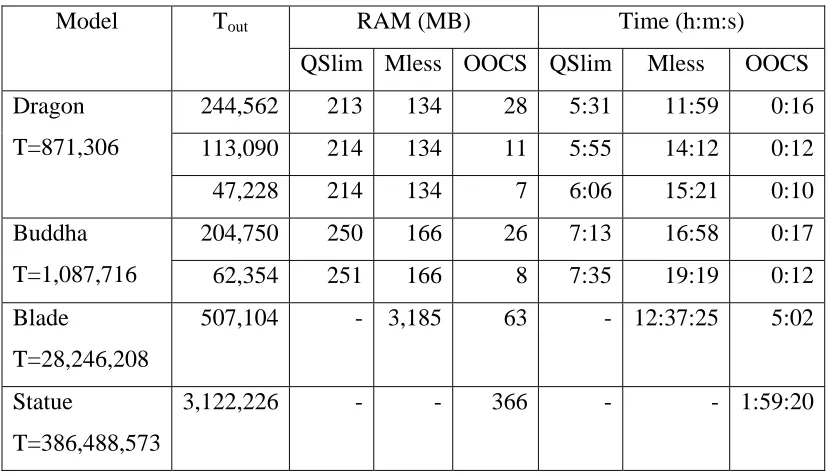
Table 2.3 Simplification results of running QSlim, memoryless simplification (Mless) and OOCS. All results were gathered on a 195 MHz R 10000 SGI Origin with 4GB of RAM and a standard SCSI disk drive (Lindstrom, 2000)
RAM (MB) Time (h:m:s)
Model Tout
QSlim Mless OOCS QSlim Mless OOCS
244,562 213 134 28 5:31 11:59 0:16
113,090 214 134 11 5:55 14:12 0:12
Dragon T=871,306
47,228 214 134 7 6:06 15:21 0:10
204,750 250 166 26 7:13 16:58 0:17
Buddha
T=1,087,716 62,354 251 166 8 7:35 19:19 0:12
Blade
T=28,246,208
507,104 - 3,185 63 - 12:37:25 5:02
Statue
T=386,488,573
3,122,226 - - 366 - - 1:59:20
simplification doesn’t retain the history of simplified mesh free up some space for this process. Nevertheless, statue with input size 400 millions of triangles cannot be processed by memoryless simplification anymore as it cannot be fit into limited RAM memory. It is not a problem for OOCS as it doesn’t depend on input mesh’s size. OOCS can process any mesh with constraint that the size of the output mesh mustn’t larger than RAM size. While being much more memory efficient, this out-of-core simplification technique also orders of magnitude faster.
OOCS is fast, but the quality is looser because it doesn’t perform adaptive sampling. Further, since OOCS does not reply on connectivity information, it has no way of detecting boundary edges (or non-manifold edge). To make the quality better, hybrid approach could be considered, that is, first, perform OOCS on a large model, then follow by slower but accurate in-core simplification (Lindstrom, 2000a).
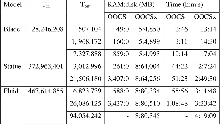
Even though OOCS can display lots of massive data, however, it encounters problem when dealing with the output size, which is larger than available main memory. Referring Table 2.4, OOCS is faster than OOCSx (Lindstrom and Silva, 2001) between two to five times when output mesh remains smaller than RAM size. But, in one case, for simplification of blade, OOCSx is faster than OOCS. The reason is OOCS ran out of memory, and numerous page faults occurred. Another case is 15.5MB RAM even is not enough for OOCS to simplify the fluid. Memory usage of OOCSx depends on size of the input mesh, whereas memory usage for OOCS is proportional to size of output mesh. Additionally, OOCSx only use arbitrary little main memory (5MB or 8MB RAM in this simplification process). Contrary, OOCS use all available main memory for displaying the output mesh.
In (Lindstrom, 2003c), Lindstrom has improved insensitive algorithm
Table 2.4 Run-time performance of OOCS and OOCSx. Blade were computed on Linux PC with 512MB RAM and two 800 MHz Pentium III processor. Statue and fluid are simplified on SGI Onyx2 with forth-eight 250MHz R10000 processor and 15.5GB RAM. (Lindstrom and Silva, 2001)
RAM:disk (MB) Time (h:m:s)
Model Tin Tout
OOCS OOCSx OOCS OOCSx
507,104 49:0 5:4,850 2:46 13:14
1, 968,172 160:0 5:4,899 3:11 14:30 Blade 28,246,208
7,327,888 859:0 5:4,993 19:14 17:04 3,012,996 261:0 8:64,004 44:22 2:7:24 Statue 372,963,401
21,506,180 3,407:0 8:64,256 51:23 2:49:30 6,823,739 588:0 8:80,334 55:56 3:11:48 26,086,125 3,427:0 8:80,510 1:08:48 3:23:42 Fluid 467,614,855
94,054,242 - 8:80,345 - 4:19:09
Simplification using Octree-based External Memory Mesh (OEMM) by (Cignoni et al., 2003c) eventually faster than in-core simplification method: QSlim and RAM-QEM (implementation of QEM in main memory) and their RMS errors are quite similar. However, it is much slower than OOCS even though the error metrics is much smaller (higher quality) than OOCS. Besides, Cignoni et al. (2003c) can produce up to 13K triangles per second, but the output is not directly usable in view-dependent refinement. Table 2.5 shows the simplification of a Happy Buddha (1,087, 716 faces) on PIII 800MHz PC with 128MB RAM.
Table 2.5 Simplification on Happy Buddha using four different codes (Cignoni et al., 2003c)
Code Simpl.
faces
RAM (MB)
Time (s) Tps rate RMS err
QSlim v2.0 18,338 195 60 17.4K 0.0131
RAM-QEM 18,338 160 58 18K 0.0125
- 4 58
-OEMM-QEM (Preprocess)
OEMM-QEM (Simplify) 18,338 60 48 21.7K 0.0129
An approach making the out-of-core simplification with a guaranteed error tolerance (Borodin et al., 2003) is implemented using vertex contraction technique instead of vertex clustering. Even the error is minimized until lower than QSlim (Garland and Heckbert, 1997) and output’s quality is high, the simplification time is relatively slow. Plus, their work doesn’t show the statistics of simplified mesh with size larger than 35K triangles (See Table 2.6).
Table 2.6 Reduction and performance rates for four standard models using a 1.8GHz Pentium IV PC with 512MB main memory (Borodin et al., 2001)
Model Tin Tout Error Simplifcation
time (h:m:s)
Rate (tps)
Armadillo 345 944 33 780 0.129 0:05:06 826
Happy Buddha 1 087 716 32 377 0.170 0:19:28 728
David 2mm 8 254 150 25 888 0.178 2:22:02 762
Lucy 28 055 742 26 772 0.163 8:03:57 779
A multiphrase approach (Garland and Shaffer, 2002), which operates by combining an initial out-of-core uniform clustering phase with a subsequent in-core iterative edge contraction phase performs very well in simplification process. This technique produces higher quality, better distribution of triangles than uniform spatial clustering. But, higher grid resolution needed in the first pass causing the more memory is consumed. Besides, it is still output sensitive. They have compared their results with OOCS (Lindstrom, 2000), adaptive out-of-core clustering (Shaffer and Garland, 2001), and QSlim (Garland and Heckbert, 1997). Results show that it is able to simplify polygonal mesh of arbitrary size, like OOCS, but it is able to generate much higher quality approximations at moderate to small output sizes. Indeed, it consistently produces approximations of quality comparable to QSlim, but using considerably less running time and memory, both asymptotically and in practice.
Their work is compared with out-of-core algorithm without crack filling and in-core rendering. The frame rates that it produced are adequate to generate an excellent real-time application probably due to the good VGA card they used.
Correa (2003) proposes a new algorithm in out-of-core simplification, consisting two phrases of work as well, which is preprocessing and runtime. In building the octree, a finer tree creates a more precise view-frustum. Coarser granularity reduces traversal time, decreases vertex replication but increases possibility of fetching and rendering of invisible geometry. LoD generations are created by vertex clustering technique. Besides, occlusion culling and sort-first parallel rendering are also implemented.
For preprocessing step, 2.4 GHz Pentium IV computer with 512 MB of RAM, 250 GB IDE disk and a NVIDIA GeForce Quadro FX 5200 Graphics card is used. During octree generation, based on his thesis’s figure, granularity of 15K vertices per leaf needs roughly six minutes to generate it. Whilst LOD generation for the original data and four simplified models needs approximately eight minutes of time with additional data size of 268MB. This algorithm is fairly good in its speed aspect. Nevertheless, due to his implementation constructs static LOD, while Lindstrom (2003c) generates view-dependent LOD, and hence comparison is hard to be made between these algorithms. Besides, no figures on simplification time are shown. Subsequently, it is difficult to compare its efficiency with other existing algorithms.
Comparison between performance of adaptive and uniform clustering
methods have been carried out by Shaffer and Garland (2001). Tool Metro (Cignoni et al., 1998) is used to measure error metrics. The results show that error in coarse approximation is reduced about 20%. At the same time, finer resolution is dropped around 10% too. This shows that adaptive gives better quality approximation. However, the time consuming to simplify the mesh is varied from around 2.5 to 3 times as much as that required for uniform clustering. As a short conclusion,
adaptive clustering induces better quality mesh but slower than uniform clustering do.