Fast, Incremental, and Scalable All Pairs Similarity Search

(1)

AWEKAR, AMIT C. Fast, Incremental, and Scalable All Pairs Similarity Search. (Under the direction of Professor Nagiza F. Samatova and Professor Anatoli V. Melechko).

Searching pairs of similar data records is an operation required for many data mining techniques like clustering and collaborative filtering. With the emergence of the Web, scale of the data has increased to several millions or billions of records. Business and scientific applications like search engines, digital libraries, and systems biology often deal with massive datasets in a high dimensional space. The overarching goal of this dissertation is to enable fast and incremental similarity search over large high dimensional datasets through improved indexing, systematic heuristic optimizations, and scalable parallelization. In Task 1, we design a sequential algorithm for All Pairs Similarity Search (AP SS) that involves finding all pairs of records having similarity above a specified threshold. Our proposed fast matching technique speeds-up AP SS computation by using novel tighter bounds for similarity computation and indexing data structure. It offers the fastest solution known to date with up to 6X speed-up over the state-of-the-art existingAP SS algorithm. In Task 2, we address the incremental formulation of the AP SS problem, where

AP SS is performed multiple times over a given dataset while varying the similarity thresh-old. Our goal is to avoid redundant computations across multiple invocations ofAP SS by storing computation history during eachAP SS. Depending on the similarity threshold vari-ation, our proposed history binning and index splitting techniques achieve speed-ups from 2X to over 105X over the state-of-the-artAP SS algorithm. To the best of our knowledge, this is the first work that addresses this problem.

In Task 3, we design scalable parallel algorithms for AP SS that take advantage of modern multi-processor, multi-core architectures to further scale-up theAP SS compu-tation. Our proposed index sharing technique divides the AP SS computation into inde-pendent tasks and achieves ideal strong scaling behavior on shared memory architectures. We also propose a complementary incremental index sharing technique, which provides a memory-efficient parallelAP SS solution while maintaining almost linear speed-up. Perfor-mance of our parallelAP SS algorithms remains consistent for datasets of various sizes. To the best of our knowledge, this is the first work that explores parallelization forAP SS.

(2)

by Amit Awekar

A dissertation submitted to the Graduate Faculty of North Carolina State University

in partial fullfillment of the requirements for the Degree of

Doctor of Philosophy

Computer Science

Raleigh, North Carolina

2009

APPROVED BY:

Professor Kemafor Anyanwu Professor Christopher G. Healey

(3)

BIOGRAPHY

(4)

ACKNOWLEDGMENTS

First, I would like to thank Professor Nagiza F. Samatova and Professor Anatoli V. Melechko, my advisors. They have been great mentors guiding me through my research. I am also indebted to Profs. Kemafor Anyanwu and Christopher G. Healey for serving on my thesis committee. I would like to thank Paul Breimyer and others in Prof. Samatova’s research group, for helping me time to time. I am also thankful to Bev Mufflemann for reviewing my dissertation draft. I want to thank my wife, Shraddha More, for all her love and trust. Finally, I am thankful to my parents, brother Ajit, and friends, for their continuous encouragement and support.

(5)

TABLE OF CONTENTS

LIST OF TABLES . . . vi

LIST OF FIGURES . . . vii

1 Introduction . . . 1

1.1 Motivations, Problems, and Contributions . . . 1

1.1.1 Serial All Pairs Similarity Search (AP SS) Algorithms . . . 3

1.1.2 IncrementalAP SS Algorithms . . . 3

1.1.3 ParallelAP SS Algorithms . . . 4

1.2 Publications . . . 5

2 Serial AP SS Algorithms . . . 6

2.1 Introduction . . . 6

2.1.1 Contributions . . . 7

2.1.2 Results . . . 8

2.2 Definitions and Notations . . . 8

2.3 Datasets . . . 9

2.4 Common Framework . . . 12

2.4.1 Preprocessing . . . 13

2.4.2 Matching . . . 13

2.4.3 Indexing . . . 14

2.5 Fast Matching . . . 14

2.5.1 Upper Bound on the Similarity Score . . . 15

2.5.2 Lower Bound on the Candidate Vector Size . . . 15

2.6 AP Time Efficient Algorithm . . . 16

2.6.1 Tighter Bounds . . . 16

2.6.2 Effect of Fast Matching on Matching Phase . . . 17

2.7 Extension to Tanimoto Coefficient . . . 18

2.8 Fast Matching Performance Evaluation . . . 18

2.9 Related Work . . . 23

2.10 Conclusion . . . 24

3 Incremental AP SS Algorithms . . . 28

3.1.2 Results . . . 31

3.1.3 IAP SSand Other Incremental Problems . . . 31

3.2 IncrementalAP SS (IAP SS) Algorithm Overview . . . 31

3.3 Booting . . . 32

(6)

3.3.2 Booting Algorithm . . . 35

3.4 Upscaling . . . 36

3.5 Downscaling . . . 40

3.5.1 Division of Search Space . . . 40

3.5.2 Index Splitting . . . 40

3.5.3 Downscaling Algorithm . . . 41

3.6 Parallelization . . . 44

3.7 End-to-End IAP SS Performance . . . 47

3.7.1 Query Responsiveness to Similarity Value Change inIAP SS . . . . 47

3.7.2 Extreme Cases Speed-up . . . 48

3.7.3 Sensitivity to VaryingPmax . . . 50

3.8 IAP SS with Reduced I/O Overhead . . . 52

3.8.1 Booting . . . 53

3.8.2 Upscaling and Downscaling . . . 55

3.8.3 Flooring . . . 55

3.8.4 Extreme Cases Speed-up . . . 56

4 Parallel AP SS Algorithms . . . 58

4.1.2 Results . . . 63

4.2 Overview of Serial AP SS Algorithms . . . 63

4.3 Index Sharing . . . 64

4.3.1 Index Metadata Replication . . . 65

4.3.2 Static Partitioning . . . 65

4.3.3 Dynamic Partitioning . . . 68

4.4 ISIM R Algorithm . . . 68

4.4.1 ISIM RAlgorithm Performance Evaluation . . . 69

4.5 Incremental Index Sharing . . . 78

4.6 IISIC Algorithm . . . 78

4.6.1 IISIC Algorithm Performance Evaluation . . . 79

(7)

LIST OF TABLES

(8)

LIST OF FIGURES

Figure 1.1 Thesis Overview . . . 2

Figure 2.1 Unifying Framework for Recent ExactAP SS Algorithms . . . 7

Figure 2.2 Distribution of Vector Sizes . . . 11

Figure 2.3 Distribution of Component Weights . . . 12

Figure 2.4 Ignored Entries from Inverted Index vs. Similarity Threshold for Cosine Similarity . . . 20

Figure 2.5 Candidate Pairs Evaluated vs Similarity Threshold for Cosine Similarity . . 21

Figure 2.6 Runtime in Seconds vs. Similarity Threshold for Cosine Similarity . . . 22

Figure 2.7 Speed-up Over All P airs Algorithm vs. Similarity Threshold for Cosine Similarity . . . 23

Figure 3.1 IAP SS Overview. . . 32

Figure 3.2 Running Time ofIAP SS for the Booting Case . . . 33

Figure 3.3 Size of Computation History for the Booting Case . . . 34

Figure 3.4 Running Time ofIAP SS for the Upscaling Case. . . 37

Figure 3.5 Speed-up ofIAP SS for the Upscaling Case . . . 38

Figure 3.6 Computation History Access Statistics for the Upscaling Case . . . 39

Figure 3.7 Parallelization Overview . . . 47

Figure 3.8 Running Time ofIAP SS for the Downscaling Case . . . 48

Figure 3.9 Speed-up ofIAP SS for the Downscaling Case . . . 49

Figure 3.10 Fraction of Matching Pairs Immediately Found by Downscaling Algorithm 50 Figure 3.11 Best and Worst Case Speed-up for Similarity Values in Set T . . . 51

(9)

Figure 3.13 Size of Computation History for Booting Case ofIAP SSwith Reduced I/O

Overhead . . . 54

Figure 4.1 Overview of Index Sharing Technique . . . 60

Figure 4.2 Overview of Incremental Index Sharing Technique . . . 62

Figure 4.3 Comparison of Various Partitioning Strategies . . . 67

Figure 4.4 Execution Time vs. Number of Processing Elements forISIM RAlgorithm and SerialAP SS Algorithms . . . 73

Figure 4.5 Speed-up OverAll P airsAlgorithm vs. Number of Processing Elements for ISIM RAlgorithm . . . 74

Figure 4.6 Speed-up Over AP T ime Ef f icient Algorithm vs. Number of Processing Elements for ISIM RAlgorithm . . . 75

Figure 4.7 Efficiency vs. Number of Processing Elements forISIM R Algorithm . . . 76

Figure 4.8 Comparison of Speed-up of ISIM R Algorithm Over AP T Algorithm for Different Dataset Sizes (n) in Multi-processor Environment . . . 77

Figure 4.9 Comparison of Efficiency ofISIM R Algorithm for Different Dataset Sizes (n) in Multi-processor Environment . . . 77

Figure 4.10 Comparison of Memory Requirements of IISIC Algorithm with AP T Al-gorithm . . . 82

Figure 4.11 Comparison of Reduction in Memory Size for Various Datasets UsingIISIC Algorithm . . . 83

Figure 4.12 Execution Time vs. Number of Processing Elements for IISIC Algorithm on Multi-Processor Machine . . . 84

(10)

Chapter 1

Introduction

1.1 Motivations, Problems, and Contributions

With the exponentially growing size of available digital data and the limited human capacity to analyze data,searchis one of the most important tools to cope with the resulting information overkill. Keyword search with a ranked output list of documents is the most popular search method from an end-user’s perspective [56]. To deliver this final result, a search system has to use various other types of search algorithms to pre-process [49, 29, 43], index [46, 45], mine [26, 76], and query [58] the data. For example,near duplicate search

is used to clean the data by eliminating data instances that are almost duplicates [33, 47]; and k-nearest neighbor search is used to find anomalies in a dataset [78].

Many real-world systems frequently have to search for all pairs of records with similarity above the specified threshold. This problem is referred as the all pairs similarity search (AP SS) [16], orsimilarity join [30]. Example applications that require one to solve theAP SS problem include, but are not limited to:

• Web search engines that suggest similar web pages to improve user experiences [32];

• Online social networks that target similar users as potential candidates for new friend-ship and collaboration [74]; and

• Digital libraries that recommend similar publications for related readings [60].

(11)

AP SS is a compute-intensive problem. Given a dataset with n records in a d -dimensional space, where n << d, the na¨ive algorithm for the AP SS will compute the similarity between all pairs in O(n2·d) time. Such a solution is not practical for datasets with millions of records, which are typical in real-world applications.

Thus, the research in this thesis is inspired by the need for the efficient treatment of theAP SS problem for emerging and growing high-dimensional, sparse, and large datasets in Web-based applications like search engines, online social networks, and digital libraries. These applications use AP SS to perform data mining tasks, such as collaborative filtering [48], near duplicate detection [72, 73, 65, 39, 40], coalition detection [62], clustering [20], and query refinement [70, 18]. Although these data mining tasks are not novel, the scale of the problem has increased dramatically, and the AP SS problem is the rate limiting factor for their practical applicability.

(12)

In summary, solving theAP SSproblem for real-world applications is computation-ally challenging. This research focuses on designing and implementing scalable algorithms for solving the AP SS problem within feasible time constraint. Please, refer to Figure 1.1 for thesis overview. Specifically, we propose the following advancements:

• Fast matching of data records in theAP SS algorithms (Section 1.1.1 and Chapter 2);

• Incremental algorithm for theAP SS problem with varying similarity thresholds (Sec-tions 1.1.2 and Chapter 3); and

• Parallel AP SS algorithm that further speeds-up AP SS computation and enables processing of even larger datasets in a feasible time (Sections 1.1.3 and Chapter 4).

Next, we briefly summarize each of these advancements.

1.1.1 Serial All Pairs Similarity Search (AP SS) Algorithms

We propose a unifying framework for existing AP SS algorithms. The framework includes the following core components:

• data preprocessing, or sorting data records and computing summary statistics;

• pairs matching, or computing similarity between selective data record pairs; and

• record indexing, or adding a part of a data record to an indexing data structure.

Within this framework, we develop the fast matching technique by deriving novel tighter bounds on similarity computation and indexing structure. We incorporate these bounds into the state-of-the-art AP SS algorithm to derive our AP T ime Ef f icient algorithm, which is the fastest-to-date serialAP SS algorithm.

Chapter 2 describes the fast matching technique and AP T ime Ef f icient algo-rithm, and empirical studies demonstrating their superior performance. This work is pub-lished in the IEEE 2009 Web Intelligence Conference [12].

1.1.2 Incremental AP SS Algorithms

(13)

to as the incremental all pairs similarity search (IAP SS), which performsAP SS multiple times on the same dataset by varying the similarity threshold value.

Existing solutions forAP SS fail to prune redundant computations across multiple invocations ofAP SS because eachAP SS is performed independently. We develop history binningandindex splitting techniques for storing and clustering computation history during each invocation ofAP SS. The size of the computation history increases quadratically with the number of records in the dataset. This may create a significant I/O bottleneck. We introduce the concept of a similarity floor to store partial computation history, resulting in reduced I/O overhead. By incorporating these techniques into AP T ime Ef f icient

algorithm, we present the first solution for theIAP SS problem that systematically prunes redundant computations.

Chapter 3 discusses our IAP SS solution. This work is published as part of the ACM KDD, 2009 Workshop on Social Network Analysis and Mining [13]. Strategy to reduce I/O overhead in incremental AP SS is published in the WorldComp 2009 International Conference on Information and Knowledge Engineering [14].

1.1.3 Parallel AP SS Algorithms

Existing solutions for AP SS are all limited to serial algorithms [71, 9, 16, 81, 79, 12]. This serial nature ofAP SS solutions is a limiting factor for applicability ofAP SS to large-scale real-world problems. Inspired by the success of parallel computing in dealing with large-scale problems [7, 67, 36, 15], we explore parallelization to further scale-upAP SS

computation.

To parallelize theAP SScomputation, we propose two complementary techniques: index sharing andincremental index sharing. Index sharing technique is designed with the goal of achieving linear speed-up over the fastest serial algorithm by dividing the AP SS

computation into independent tasks. However, for large datasets, the memory requirement of AP SS might exceed the amount of main memory available. Incremental index sharing technique is designed to provide a memory-efficient parallelAP SS solution while maintain-ing almost linear speed-up over the fastest serial algorithm.

(14)

1.2 Publications

1. Title: Incremental All Pairs Similarity Search for Varying Similarity Thresholds with Reduced I/O Overhead [14]

The International Conference on Information and Knowledge Engineering, 2009. IKE ’09, July 13-17, Las Vegas, Nevada, USA, (687-693).

Authors: Amit Awekar, Nagiza F. Samatova, and Paul Breimyer

2. Title: Incremental All Pairs Similarity Search for Varying Similarity Thresholds [13] The 13th ACM SIGKDD International Conference on Knowledge Discovery and Data Mining, the Third Workshop on Social Network Mining and Analysis, 2009. SNAKDD ’09, June 28, Paris, France.

Authors: Amit Awekar, Nagiza F. Samatova, and Paul Breimyer

3. Title: Fast Matching for All Pairs Similarity Search [12]

The IEEE/WIC/ACM International Conference on Web Intelligence and Intelligent Agent Technology, 2009. WI-IAT ’09, September 15-18, Milan, Italy, (295-300). Authors: Amit Awekarand Nagiza F. Samatova

4. Title: Selective Approach to Handling Topic Oriented Tasks on the World Wide Web [10]

The IEEE Symposium on Computational Intelligence and Data Mining, 2007. CIDM ’07, April 1-5, Honolulu, Hawaii, USA, (343-348).

Authors: Amit Awekarand Jaewoo Kang

5. Title: Selective Hypertext Induced Topic Search [11]

The 15thInternational Conference on World Wide Web, 2006. WWW ’06, May 23-26, Edinburg, Scotland, (1024-1024).

(15)

Chapter 2

Serial

AP SS

Algorithms

2.1 Introduction

In this chapter, we present AP T ime Ef f icient algorithm, which is the fastest serial algorithm for All Pairs Similarity Search (AP SS). Our algorithm uses fast matching technique that is based on novel tighter bounds for similarity computation and indexing data structure.

AP SS is a compute-intensive problem. Given a data set with n records in a d -dimensional space, where n << d, the na¨ıve algorithm for the AP SS will compute the similarity between all pairs in O(n2 ·d) time. Such a solution is not practical for data sets with millions of records, which are typical in real-world applications. Therefore, many

heuristic solutions based on hashing [44, 28], shingling [23], or dimensionality reduction [51, 37] have been proposed to address this problem (please, refer to Section 2.9 for related work).

However, recent exactalgorithms for theAP SS [71, 9, 16, 81, 79] have performed even faster than the heuristic methods because of their ability to significantly prune the similarity score computation by taking advantage of the fact that only a small fraction of all Θ(n2) pairs typically satisfy the specified similarity threshold. These exact algorithms depend on theinverted index, which maps each dimension to the list of records with non-zero projection along that dimension.

(16)

• data preprocessing, or sorting data records and computing summary statistics;

• pairs matching, or computing similarity between selective data record pairs; and

• record indexing, or adding a part of data record to an indexing data structure.

Figure 2.1: Unifying Framework for Recent ExactAP SS Algorithms

Please, refer to Figure 2.1 for the framework overview. The preprocessing phase reorders the records and the components within each record based on some specified sort order, such as the maximum value or the number of non-zero components in the record. The matching phase identifies, for a given record, corresponding pairs with similarity above the threshold by querying the inverted index. The indexing phase then updates the inverted index with a part of the query record. The matching and indexing phases rely on filtering conditions and heuristic optimizations derived from the ordered records and components within each record.

The matching phase dominates the computational time. It searches for similar pairs in the inverted index and computes similarity score of pairs found. Therefore, improv-ing the performance of any solution to theAP SS would require optimization of these two tasks in the matching phase.

2.1.1 Contributions

(17)

space is defined as the actual number of record pairs evaluated by the algorithm. The proposed matching incorporates the following bounds:

• the lower bound on the number of non-zero components in any record, and

• the upper bound on the similarity score for any record pair.

The former allows for reducing the number of pairs that need to be evaluated, while the latter prunes, or only partially computes, the similarity score for many candidate pairs. Both bounds require only constant computation time. We integrate our fast match-ing technique with the fastest-to-date All P airs algorithm [16] to derive the proposed

AP T ime Ef f icientalgorithm.

2.1.2 Results

We conduct extensive empirical studies using four real-world million record data sets described in Section 2.3. We compare the performance of our AP T ime Ef f icient

algorithm against the state-of-the-art All P airs algorithm [16] using two frequently used similarity measures: the cosine similarity and the Tanimoto coefficient. We achieve up to 6X speed up in our experiments, while reducing the search space by at least an order of magnitude.

2.2 Definitions and Notations

In this section, we define the AP SS problem and other important terms referred throughout the thesis (please, see Table 2.1 for the summary of notations).

Definition 1 (All Pairs Similarity Search): The all pairs similarity search (AP SS) problem is to find all pairs (x, y) and their exact value of similarity sim(x, y) such that

x, y∈V and sim(x, y) ≥t, where

• V is a set ofnreal valued, non-negative, sparse vectors over a finite set of dimensions

Dand |D|=d;

• sim(x, y) :V ×V →[0,1] is a symmetric similarity function; and

(18)

Definition 2 (Inverted Index): The inverted index maps each dimension to a list of vectors with non-zero projections along that dimension. A set of alldlistsI ={I1, I2, ..., Id}, i.e., one for each dimension, represents the inverted index for V. Each entry in the list has a pair of values (x, w) such that if (x, w)∈Ik, then x[k] = w.

Definition 3 (Candidate Vector and Candidate Pair):

Given a vector x∈V, any vectory in the inverted index is a candidate vector, if ∃j such thatx[j]>0 and (y, y[j])∈Ij. The corresponding pair (x, y) is a candidate pair.

Definition 4 (Matching Vector andMatching Pair): Given a vectorx∈V and the similarity threshold t, a candidate vectory∈V is a matching vector forx ifsim(x, y)≥t. The corresponding pair (x, y) is a matching pair.

During subsequent discussions we assume that all vectors are of unit length (||x||= ||y|| = 1), and the similarity function is the cosine similarity. In this case, the cosine similarity equals the dot product, namely:

sim(x, y) =cos(x, y) =dot(x, y).

Our algorithms can be extended to other popular similarity measures like the Tanimoto coefficient and the Jaccard similarity using transformations presented in Section 2.7.

2.3 Datasets

(19)

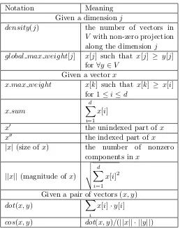
Table 2.1: Notations Used

Notation Meaning

Given a dimensionj

density(j) the number of vectors in

V with non-zero projection along the dimensionj global max weight[j] x[j] such that x[j] ≥ y[j]

for∀y∈V

Given a vectorx

x.max weight x[k] such that x[k] ≥ x[i] for 1≤i≤d

x.sum

d

X

i=1 x[i]

x0 the unindexed part ofx

x00 the indexed part ofx

|x|(size ofx) the number of nonzero components inx

||x||(magnitude of x)

v u u t

d

X

i=1 x[i]2

Given a pair of vectors (x, y)

dot(x, y) X

i

x[i]·y[i]

cos(x, y) dot(x, y)/(||x|| · ||y||)

Table 2.2: Datasets Used

Dataset n=d Total Non-zero Average Components Size Medline 1565145 18722422 11.96

(20)

1 10 100 1000 10000 100000 1e+06

1 10 100 1000 10000

Frequency Vector Size Medline 1 10 100 1000 10000 100000 1e+06

1 10 100 1000 10000 100000

Frequency Vector Size Flickr 1 10 100 1000 10000 100000 1e+06

1 10 100 1000 10000

Frequency Vector Size LiveJournal 1 10 100 1000 10000 100000

1 10 100 1000 10000 100000

Frequency

Vector Size Orkut

Figure 2.2: Distribution of Vector Sizes

Medline

(21)

0.05

0.1

0.15

0.2

0.25

0.5

0.75 Probability

Weight of component

Medline

Figure 2.3: Distribution of Component Weights

Flickr, LiveJournal, and Orkut

These three datasets were selected to explore potential applications for large on-line social networks. We are interested in finding user pairs with similar social networking patterns. Such pairs are used to generate more effective recommendations based on collab-orative filtering [74]. We use the dataset prepared by Misloveet al. [64]. Every user in the social network is represented by a vector over the space of all users. A user’s vector has non-zero projection along those dimensions that correspond to the users in his/her friend list. But the weights of these social network links are unknown. So, we applied the weight distribution from the Medline dataset to assign the weights to these social network links in the two datasets (please, refer to Figure 2.3). To ensure that our results are not specific only to the selected weight distribution, we also conducted experiments by generating the weights randomly. The results were similar and are available on the Web for downloading [1].

2.4 Common Framework

(22)

the inverted index. Most of the time, however, the information retrieval system requires only top-k similar pairs [68, 69], while the AP SS requires all matching pairs. The framework can be broadly divided into three phases: data preprocessing, pairs matching, and indexing (please, refer to Algorithm 1 for details).

2.4.1 Preprocessing

The preprocessing phase reorders vectors using a permutation Ω defined over V

(lines 1-5, Algorithm 1). Bayardo et al. [16] and Xiao et al. [81] sorted vectors on the maximum value within each vector. Sarawagi et al. [71] sorted vectors on their size. The components within each vector are also rearranged using a permutation Π defined overD. Bayardoet al. [16] observed that sorting the dimensions inDbased on vector density speeds up the AP SS. The summary statistics about each record, such as its size, magnitude, and maximum component value are computed during the preprocessing phase. They are used later to derive filtering conditions during the matching and indexing phases to save time and memory. The time spent on preprocessing is negligible compared to the time spent on matching.

2.4.2 Matching

The matching phase scans the lists in the inverted index that correspond to the non-zero dimensions in x, for a given vector x ∈ V, to find candidate pairs (lines 7-16, Algorithm 1). Simultaneously, it accumulates a partial similarity score for each candidate pair. Bayardoet al. [16] and Xiaoet al. [81] used the hash-based map, while Sarawagi et al. [71] used the heap-based scheme for score accumulation.

Given t, Ω, Π andsummary statistics, various filtering conditions are derived to eliminate candidate pairs that will definitely not satisfy the required similarity threshold; these pairs are not added to the setC (line 7, Algorithm 1). Sarawagi et al. [71] identified the part of the given vector x ∈ V such that for any candidate vector y ∈ V to have

sim(x, y) ≥t, the intersection ofy with that part must be non-empty. Bayardoet al. [16] computed a lower bound on the size of any candidate vector to match with the current vector as well as any remaining vector. Our fast matching technique further tightens this lower bound.

(23)

on the similarity score in constant computational time. Xiaoet al. [81] used the Hamming distance based method for computing such an upper bound. Bayardo et al. [16] used the vector size and maximum component value to derive a constant time upper bound. We further tighten this upper bound in our fast matching technique. Finally, the exact similarity score is computed for the remaining candidate pairs, and those having scores above the specified threshold are added to the output set.

2.4.3 Indexing

The indexing phase adds a part of the given vector to the inverted index so that it can be matched with any of the remaining vectors (lines 17-21, Algorithm 1). Sarawagi et al. [71] unconditionally indexed every component of each vector. Instead of building the inverted index incrementally, they built the complete inverted index beforehand. Bayardo et al. [16] and Xiaoet al. [81] used the upper bound on the possible similarity score with only the part of the current vector. Once this bound reached the similarity threshold, the remaining vector components were indexed.

2.5 Fast Matching

In the framework described in Algorithm 1, the matching phase evaluates O(n2) candidate pairs. This phase is critical for the running time. The computation time of the matching phase can be reduced in three ways:

• traversing the inverted index faster while searching for candidate pairs,

• generating fewer candidate pairs for evaluation, and

• reducing the number of candidate pairs that are evaluated completely.

(24)

2.5.1 Upper Bound on the Similarity Score

Given a candidate pair (x, y), the following constant time upper bound on the cosine similarity holds:

cos(x, y)≤x.max weight∗y.sum. (2.1)

The correctness of this upper bound can be derived from:

x.max weight∗sum(y)≥dot(x, y) =cos(x, y). Similarly following upper bound can be derived:

cos(x, y)≤y.max weight∗x.sum. (2.2)

Combining upper bounds in 2.1 and 2.2, we propose following upper bound on cosine similarity score:

min(x.max weight∗y.sum, y.max weight∗x.sum), (2.3)

wheremin function selects minimum of the two arguments.

We can safely prune the exact dot product computation of a candidate pair if it does not satisfy the similarity threshold even for this upper bound.

2.5.2 Lower Bound on the Candidate Vector Size For any candidate pair (x, y), the following is true:

x.max weight∗y.sum≥dot(x, y).

For this candidate pair to qualify as a matching pair, the following inequality must hold:

y.sum≥t/x.max weight. For any unit-length vectory, the following is true:

y.sum≥k→ |y| ≥k2.

This gives us the following lower bound on the size of any candidate vectory:

|y| ≥(t/x.max weight)2. (2.4)

(25)

2.6 AP Time Efficient Algorithm

The proposed AP T ime Ef f icient algorithm integrates both optimizations for the lower and upper bounds with the fastest-to-dateAll P airsalgorithm [16] (please, refer to Algorithm 2). The vectors are sorted in decreasing order of their max weight, and the dimensions are sorted in decreasing order of their vector density. For every x ∈ V, the algorithm first finds its matching pairs from the inverted index (Matching Phase, Lines 6-15) and then adds selective parts ofx to the inverted index (Indexing Phase, Lines 16-22). The difference between the algorithmsAP T ime Ef f icientand All P airsis in the tighter bounds on filtering conditions. The correctness of these tighter bounds is proven above. Hence, the correctness of the AP T ime Ef f icient is the same as the correctness of the

All P airs algorithm [16].

2.6.1 Tighter Bounds

The All P airs algorithm uses t/x.max weight as the lower bound on the size of any candidate vector. TheAP T ime Ef f icientalgorithm tightens this bound by squaring the same ratio (Line 2, Algorithm 3).

TheAll P airsalgorithm uses the following constant time upper bound on the dot product of any candidate pair (x, y):

min(|x|,|y|)∗x.max weight∗y.max weight. (2.5)

We will consider following two possible cases to prove that our bound proposed in 2.3 is tighter than this bound.

1. Case 1: |x| ≤ |y|

The upper bound in 2.5 reduces to:

|x| ∗x.max weight∗y.max weight.

The upper bound proposed in 2.2 is tighter than this bound because:

x.sum≤ |x| ∗x.max weight

2. Case 2: |x|>|y|

(26)

|y| ∗x.max weight∗y.max weight.

The upper bound proposed in 2.1 is tighter than this bound because:

y.sum≤ |y| ∗y.max weight

Hence, our upper bound proposed in 2.3 on the cosine similarity (Line 9, Algorithm 2) is tighter than the existing bound.

2.6.2 Effect of Fast Matching on Matching Phase

For a given vectorx, the lower bound on the size of a candidate vector is inversely proportional tox.max weight. The vectors are sorted in decreasing order by max weight. Hence, the value of the lower bound on the size of the candidate increases monotonically as the vectors are processed. If a vectory does not satisfy the lower bound on the size for the current vector, then it will not satisfy this bound for any of the remaining vectors. Such vectors can be discarded from the inverted index.

Like All P airs, our implementation uses arrays for representing lists in the in-verted index. Deleting an element from the beginning of a list will have linear time over-head. Instead of actually deleting such entries, we just ignore these entries by removing them from the front of the list (Line 4, Algorithm 3). Because of our tighter lower bound on the size of the candidate, more such entries from the inverted index are ignored. This reduces the effective size of the inverted index, thus, resulting in faster traversal of the in-verted index during the finding of the candidate pairs. AP T ime Ef f icientalso generates fewer candidate pairs as fewer vectors qualify to be candidate vectors because of the tighter lower bound on their size.

Computing the exact dot product for a candidate pair requires linear traversal of both vectors in the candidate pair (Line 10, Algorithm 2). The tighter constant time upper bound on the similarity score of a candidate pair prunes the exact dot product computation for a large number of candidate pairs. In our experiments we observed that

AP T ime Ef f icient reduces the search space by up to two orders of magnitude (please, refer to Figure 2.5).

(27)

because our optimizations depend on the variation in the values of different components within a given vector.

2.7 Extension to Tanimoto Coefficient

In this section, we extendAP T ime Ef f icientalgorithm for the Tanimoto coeffi-cient, which is similar to the extended Jaccard coefficient for binary vectors. Given a vector pair (x, y), the Tanimoto coefficient is defined as:

τ(x, y) =dot(x, y)/(||x||2₊_||_y_||2₋_dot₍_{x, y}_)).

First, we will show that τ(x, y) ≤ cos(x, y). Without loss of generality, let ||x|| = a· ||y|| and a≥1. By definition, it follows that:

cos(x, y)/τ(x, y) = (||x||2₊_||_y_||2₋_dot₍_{x, y}₎₎_/₍_||_x_{|| ∗ ||}_y_||_),

= (a2+ 1)/a−cos(x, y), ≥(a2+ 1)/a−1,

≥1 + (a−1)2/a, ≥1.

Given the similarity threshold tfor the Tanimoto coefficient, if we run both of our algorithms with the same threshold value for the cosine similarity, then they will not filter out any matching pairs. The only change we have to make is to replace the final similarity computation (Line 10 of Algorithms 2) with the actual Tanimoto coefficient computation as follows:

s=τ(x, y).

2.8 Fast Matching Performance Evaluation

(28)

All our implementations are in C++. We used the standard template library for most of the data structures. We used the dense hash map class from GoogleT M for the hash-based partial score accumulation [3]. The code was compiled using the GNUgcc4.2.4 compiler with −O3 option for optimization. All the experiments were performed on the same 3 GHz Pentium-4 machine with 6 GB of main memory. The code and the data sets are available for download on the Web [1].

We evaluate the performance of fast matching in the AP T ime Ef f icient algo-rithm based on three parameters:

• the size of the inverted index,

• the size of the search space, and

• the end-to-end run-time.

The preprocessing phase is identical in both algorithms. The time spent on data preprocess-ing was negligible as compared to the experiments’ runnpreprocess-ing time, and was ignored. Though the indexing phase is also identical in both algorithms, the time spent in indexing phase was considered in the end-to-end running time, as it was not negligible.

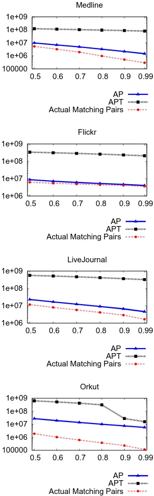
The number of entries in the inverted index ignored by AP T ime Ef f icient is two to eight times that of All P airs (please, refer to Figure 2.4). This reduction provides two-fold benefits: faster traversal of the inverted index and fewer candidate pairs evalu-ated. The memory footprints of AP T ime Ef f icientandAll P airs are the same because

AP T ime Ef f icient only ignores more entries from the inverted index, but does not re-move them from memory. The AP T ime Ef f icientreduces the search space by at least an order of magnitude (please, refer to Figure 2.5). Finally, the end-to-end speed up is up to 6X (please, refer to Figures 2.6 and 2.7). Even though the search space is reduced by an order of magnitude, we get comparatively less end-to-end speed up, because some time is still spent traversing the inverted index to find candidate pairs and filtering out a large fraction of them.

The best speed up is obtained for the Flickr data set, because it has a heavy tail in the distribution of vector sizes (please, refer to Figure 2.7). Vectors having the long size typically generate a large number of candidate pairs. But AP T ime Ef f icient

(29)

10000 100000 1e+06

0.5 0.6 0.7 0.8 0.9 0.99 Medline

AP APT

100000 1e+06 1e+07

0.5 0.6 0.7 0.8 0.9 0.99 Flickr

AP APT

100000 1e+06 1e+07

0.5 0.6 0.7 0.8 0.9 0.99 LiveJournal

AP APT

100000 1e+06 1e+07 1e+08

0.5 0.6 0.7 0.8 0.9 0.99 Orkut

AP APT

(30)

100000 1e+06 1e+07 1e+08 1e+09

0.5 0.6 0.7 0.8 0.9 0.99 Medline

AP APT Actual Matching Pairs

1e+06 1e+07 1e+08 1e+09

0.5 0.6 0.7 0.8 0.9 0.99 Flickr

1e+06 1e+07 1e+08 1e+09

0.5 0.6 0.7 0.8 0.9 0.99 LiveJournal

100000 1e+06 1e+07 1e+08 1e+09

0.5 0.6 0.7 0.8 0.9 0.99 Orkut

(31)

50 100 150 200 250 300

0.5 0.6 0.7 0.8 0.9 0.99 Medline

AP APT

0 100 200 300 400 500 600

0.5 0.6 0.7 0.8 0.9 0.99 Flickr

AP APT

200 300 400 500 600 700 800 900

0.5 0.6 0.7 0.8 0.9 0.99 LiveJournal

AP APT

1000 2000 3000 4000 5000 6000 7000 8000

0.5 0.6 0.7 0.8 0.9 0.99 Orkut

AP APT

(32)

1.5 2 2.5 3 3.5 4 4.5 5 5.5 6

0.5 0.6 0.7 0.8 0.9 0.99

Medline

Medline Flickr

LiveJournal Orkut

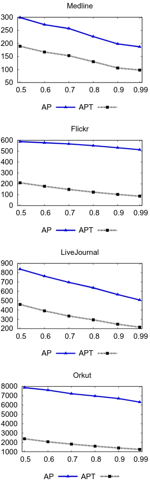
Figure 2.7: Speed-up OverAll P airs Algorithm vs. Similarity Threshold for Cosine Simi-larity

of candidate pairs evaluated by AP T ime Ef f icient almost equals the actual number of matching pairs (please refer to Figure 2.5).

2.9 Related Work

Previous work on all pairs similarity search can be divided into two main cate-gories: heuristic and exact. Main techniques employed by heuristic algorithms are hashing, shingling, and dimensionality reduction. Charikar [28] defines a hashing scheme as a dis-tribution on a family of hash functions operating on a collection of vectors. For any two vectors, the probability that their hash values will be equal is proportional to their simi-larity. Fagin et al. [37] combined similarity scores from various voters, where each voter computes similarity using the projection of each vector on a random line. Broderet al. [23] use shingles and discard the most frequent features. Li et al. [59] use approximate string matching algorithms to evaluate similarity between tree structured data.

(33)

reduce the computation time. Arasuet al. [9] generate signatures of input vectors and find pairs that have overlapping signatures. Finally, they output only those pairs that satisfy the similarity threshold. Xiao et al. [81] propose optimizations based on the length and Hamming distance specific to binary vectors. Xiao et al. [79] speed up similarity search based on edit distance measure for binary vectors. Bayardo et al. [16] propose various optimizations that employ the similarity threshold and sort order of the data, while finding matches and building the inverted index.

2.10 Conclusion

(34)

Algorithm 1: Inverted Index Based Unifying Framework for Recent Exact

AP SS Algorithms

Input: V,t,D,sim, Ω, Π

Output: M AT CHIN G P AIRS SET

M AT CHIN G P AIRS SET = ∅;

1

Ii = ∅ ,∀ 1≤i≤d;

2

/* The inverted index is initialized to d empty lists. */

Arrange vectors inV in the order defined by Ω;

3

Arrange components in each vector in the order defined by Π;

4

Compute summary statistics;

5

foreach x∈V using the order defined by Ωdo

6

C = set of candidate pairs corresponding tox, found by querying and

7

manipulating the inverted indexI; foreachcandidate pair (x, y)∈C do

8

sim max possible= upper bound onsim(x, y);

9

if sim max possible≥tthen

10

sim actual=sim(x, y);

11

if sim actual≥t then

12

M AT CHIN G P AIRS SET =

13

M AT CHIN G P AIRS SET ∪(x, y, sim actual)

14

15

foreachi such thatx[i]>0 using the order defined by Π do

16

if f iltering condition(x[i]) is true then

17

Add (x, x[i]) to the inverted index;

18

19

20

(35)

Algorithm 2: AP T ime Ef f icientAlgorithm. Input: V,t,d,global max weight, Ω, Π Output: M P S (Matching Pairs Set)

M P S = ∅;

1

Ii = ∅ ,∀ 1≤i≤d;

2

Ω sorts vectors in decreasing order by max weight;

3

Π sorts dimensions in decreasing order by density;

4

foreach x∈V in the order defined by Ωdo

5

partScoreM ap = ∅;

6

/* Empty map from vector id to partial similarity score */

FindCandidates(x, I, t,Π, partScoreM ap);

7

foreachy: partScoreM ap{y}>0do

8

if partScoreM ap{y} + sum(y)∗x.max weight≥tthen

9

/* Tighter upper bound on the similarity score */

s = partScoreM ap{y} + dot(x, y0);

10

if s≥tthen

11

M AT CHIN G P AIRS SET =

12

M AT CHIN G P AIRS SET ∪(x, y, s)

13

14

maxP roduct = 0;

15

foreachi: x[i]>0, in the order defined by Π do

16

maxP roduct=

17

maxP roduct+x[i]∗min(global max weight[i], x.max weight); if maxP roduct≥tthen

18

Ii = Ii∪ {x, x[i]};

19

x[i] = 0;

20

21

22

(36)

Algorithm 3: F indCandidatesAlgorithm. Input: x,I,t, Π,partScoreM ap

Output: modifiedpartScoreM ap, and I

remM axScore =

d

X

i=1

x[i]∗global max weight[i];

1

minSize = (t/x.max weight)2;

2

/* Tighter lower bound on candidate size */

foreach i: x[i]>0, in the reverse order defined by Π do

3

Iteratively remove (y, y[i]) from front ofIi while |y|< minSize;

4

foreach(y, y[i])∈Ii do

5

if partScoreM ap{y}>0 or remM axScore≥t then

6

partScoreM ap{y} = partScoreM ap{y} + x[i]∗y[i];

7

8

remM axScore = remM axScore − global maximum weight[i]∗x[i];

9

/* Remaining maximum score that can be added after processing

current dimension */

(37)

Chapter 3

Incremental

AP SS

Algorithms

3.1 Introduction

In Chapter 2, we presentedAP SSalgorithms for a fixed similarity threshold value. However, selecting a meaningful similarity threshold for all pairs similarity search (AP SS) is an art because it is data dependent. Domain experts often use a trial-and-error approach by looking at the quality of output. For example, the Jarvis-Patrick clustering algorithm sparsifies the similarity score matrix by retaining only those entries that satisfy a predefined threshold [52]. The optimal threshold for sparsifying the similarity score matrix can be determined only after evaluating the quality of different clusterings by varying the similarity threshold for sparsification.

Varying the similarity threshold leads to another important problem that we refer to as the incremental all pairs similarity search (IAP SS) that performs AP SS multiple times on the same dataset by varying the similarity threshold value. The IAP SS problem is challenging to solve when it is applied frequently or over large datasets. For example, to detect near duplicate documents [81], a news search engine has to solve the IAP SSproble every few minutes over a small subset of the web, whereas a web search engine has to solve theIAP SS problem once every few days, but over the entire web.

To the best of our knowledge, the IAP SS problem has not received a special treatment in scientific literature and the “brute-force” strategy is used instead [80]. Namely, applying a new instance ofAP SS after each similarity threshold value changes. Obviously, this solution may be inefficient due to inherent redundancies.

(38)

significant part of the computation is redundant across multiple invocations of AP SS, be-cause each of theAP SS instances executes independently for changing similarity threshold values. For example, consider performingAP SS twice on a dataset. Initially, the threshold value is 0.9 and later it is reduced to 0.8. All pairs present in the output of the firstAP SS

will also exist in the output of the second AP SS. There is no need to compute the simi-larity score for these pairs during the second AP SS. While executing the firstAP SS, the similarity score computed for some pairs would be less than 0.8. We can safely prune the similarity score computations of such pairs during the second AP SS. Arguably, the more timesAP SS is performed, the greater the opportunity to optimize the search by eliminating redundant calculations.

For a dataset with n records in a d dimensional space where d >> n, a brute-force algorithm for IAP SS will compute the similarity scores between all possible O(n2) pairs during each of the s selections for the similarity threshold value. As each similarity computation requiresO(d) time, the total time complexity will be O(n2∗s∗d). However, this computational cost becomes prohibitively expensive for large-scale problems. To ad-dress this limitation our solution to the IAP SS problem stores the computation history during each invocation ofIAP SS and later uses the history to systematically identify and effectively prune redundant computations. The compute and I/O intensive nature of the

IAP SS problem raises two key research challenges:

• developing efficient I/O techniques to deal with possibly large history data; and

• efficiently identifying and pruning redundant computations.

To address these challenges, we propose two major techniques: history binning and index splitting.

The history binning technique stores information about all pairs evaluated in the current invocation ofIAP SS. Pairs are grouped based on their similarity scores and stored in binary files. This information is used in the next invocation of IAP SS to avoid re-computation of known similarity scores. Grouping pairs enables our algorithm to read only the necessary parts of the computation history. The I/O for history binning is performed in parallel to the similarity score computation, which reduces the overhead in end-to-end execution time.

The index splitting technique divides the inverted index based on the values of

(39)

of the inverted index and to prune similarity score computations of pairs that exist in the computation history.

Lowering the value of the similarity threshold results in exploring a greater portion of the search space (i.e., the number of record pairs evaluated). The lowest similarity threshold value used in previous IAP SS invocations defines the parts of the search space that have already been explored. Depending on the value of the current similarity threshold (tnew) and the previous lowest similarity threshold value (told), we identify three different cases for theIAP SS problem:

1. booting, where theIAP SSalgorithm is executed for the first time on a given dataset, 2. upscaling, wheretold≤tnew, and

3. downscaling, where told> tnew.

The history binning technique is used in all three cases, while index splitting is required only for the downscaling case.

3.1.1 Contributions

We incorporate both history binning and index splitting intoAP T ime Ef f icient

algorithm, which is the state-of-the-art AP SS algorithm [12]. This incorporation enables us to split theIAP SScomputation into various independent subtasks that can be executed in parallel. This chapter proposes the following contributions:

• Develops history binning and index splitting techniques that systematically identify and effectively prune redundant computations across multiple invocations of AP SS.

• Incorporates our history binning and index splitting techniques into the state-of-the-artAP SS algorithm and parallelizes it, which leads to efficient end-to-end computa-tion.

(40)

3.1.2 Results

We perform empirical studies using four real-world million record datasets de-scribed in Section 2.3. All experiments were performed on a 2.6 GHz IntelT M XeonT M class machine with eight CPU cores and 16 GB of main memory. We compare the per-formance of our algorithm against the All P airs algorithm [16] and AP T ime Ef f icient

algorithm [12]. Depending on the similarity threshold variation, our speed-ups vary from 2X to over 105X.

3.1.3 IAP SS and Other Incremental Problems

TheIAP SSproblem should not be confused with other formulations of incremen-tal problems. Incremenincremen-tal algorithms for various types of similarity searches have primarily addressed the challenge of handling perturbations in datasets themselves, when data records and/or their dimensions are added or removed [82]. Unlike these incremental methods, the IAPSS problem assumes that such datasets remained unchanged across different searches. Some incremental algorithms are designed to identify the top-k similar pairs [27, 83, 80]. But the IAP SS problem requires all matching pairs. Incremental algorithms for the dis-tance join [50, 61] address problems similar to IAP SS for distance measures, such as the Euclidian distance. However, their techniques assume that the triangle inequality holds true for distance measures, which is not the case for similarity functions like the cosine similarity and the Tanimoto coefficient.

3.2 Incremental

AP SS

(IAP SS

) Algorithm Overview

The IAP SS problem is to the solve the AP SS problem for a given similarity threshold value tnew when the AP SS problem has already been solved for the previous value of similarity threshold told. The IAP SS algorithm is based on the observation that the proportion of the search space explored during the execution of a singleAP SSinvocation is inversely proportional to the value of the similarity threshold. If t < t0, then the search space explored while executing AP SS for t0 is a subset of the search space explored for

(41)

an overview of the IAP SS algorithm and there are three possible cases for the IAP SS

solution:

Figure 3.1: IAP SS Overview

1. Booting: told = ∞, executing the IAP SS algorithm for the first time on a given dataset.

2. Upscaling: told ≤ tnew, reading a subset of pairs that are already present in the computation history.

3. Downscaling: told> tnew, potentially adding new similarity pairs to the computation history.

3.3 Booting

(42)

3.3.1 History Binning

Our IAP SS algorithm takes a user defined parameter, Pmax, that specifies the number of partitions for the similarity interval of [0,1]. The interval is divided into equal sized non-overlappingPmaxpartitions. For example, ifPmax = 5, then the similarity interval is divided into five partitions: [0,0.2); [0.2,0.4); [0.4,0.6); [0.6,0.8); and [0.8,1.0]. Given a similarity value s, the corresponding partition number Ps can be calculated in constant time asPs =bs∗Pmaxc. For the special case ofs= 1 the partition number isPmax−1. All experiments reported in this paper are performed with Pmax = 20. The effect of varying

Pmax is discussed in Section 3.7.3.

10 100 1000 10000

0.5 0.6 0.7 0.8 0.9 0.99

Time in Seconds

Booting Similarity Threshold

Medline Flickr

LiveJournal Orkut

Figure 3.2: Running Time ofIAP SS for the Booting Case

(43)

100 1000 10000 100000

0.5 0.6 0.7 0.8 0.9 0.99

Size in MB

Booting Similarity Threshold

Medline Flickr

LiveJournal Orkut

Figure 3.3: Size of Computation History for the Booting Case

3.3.2 Booting Algorithm

Booting is the case of executing theIAP SSalgorithm for the first time on a given dataset. As there is no information available from any previous invocation of AP SS, our

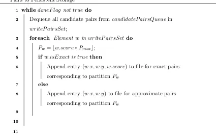
IAP SS algorithm simply uses the fastest algorithm forAP SS while storing the computa-tion history. The booting algorithm is divided into two concurrent threads: the Candidate Pair Producer and the Candidate Pair Consumer. The Candidate Pair Producer executes theAll P airs algorithm (please, refer to Algorithm 4), and the Candidate Pair Consumer writes candidate pairs to persistent storage (please, refer to Algorithm 5).

The producer and consumer share two data structures: thedoneF lagandcandidat eP airQueue. The doneF lag is a binary variable that is initialized to false, and the Can-didate pair producer sets it to true when all candidate pairs are added to the candidate P airQueue. Each entry in the candidateP airQueuehas four components: the ids of both vectors in the pair, the similarity score value, and a flag indicating if it is the exact score or an upper bound.

(44)

Algorithm 4: Candidate P air P roducer Algorithm: Replace lines 9-13 of Algorithm 2 with the Following Pseudocode

upperBound=

1

partScoreM ap{y} + min(sum(y0)∗x.max weight, sum(x)∗y0.max weight); if upperBound≥tthen

2

3

Add (x, y, s, true) to candidateP airQueue;

4

if s≥t then

5

M P S =M P S ∪ (x, y, s)

6

7

else

8

Add (x, y, upperBound, f alse) to candidateP airQueue;

9

10

Figure 3.2 shows the running time of the IAP SS booting algorithm for various similarity threshold values. Performance of IAP SSfor the booting case is the same as the

AP T ime Ef f icientalgorithm.

3.4 Upscaling

Upscaling is another simple case of IAP SS, which only requires reading a part of the computation history and is the case where told ≤ tnew. The set of matching pairs for threshold tnew will be a subset of the matching pairs for told. The matching pairs for

told are a subset of all the candidate pairs for threshold told and have already been stored through history binning while executing IAP SS fortold. If a pair is a matching pair, then its similarity score is computed exactly (lines 3-7, Algorithm 4). Therefore, all matching pairs for threshold told have already been stored in exact pairs files. No separate search is required to find the matching pairs for threshold tnew.

(45)

Algorithm 5: Candidate P air ConsumerAlgorithm for Writing Candidate Pairs to Persistent Storage

while doneF lag not truedo

1

Dequeue all candidate pairs fromcandidateP airsQueue in

2

writeP airsSet;

foreach Element w in writeP airsSet do

3

Pw =bw.score∗Pmaxc;

4

if w.isExact istrue then

5

Append entry (w.x, w.y, w.score) to file for exact pairs

6

corresponding to partitionPw else

7

Append entry (w.x, w.y) to file for approximate pairs

8

corresponding to partitionPw

9

10

11

and then reads the exact pairs files corresponding to all partitions P, Pnew ≤ P < Pmax. The pairs satisfying the threshold tnew are then added to the output.

During our experiments, the first IAP SS (booting) experiment used a thresh-old value of 0.5 and then performed upscaling with various similarity thresholds. For all datasets, upscaling was completed in less than two seconds (please, refer to Figure 3.4); this is expected because the algorithm only reads and outputs matching pairs. It results in large speed-ups in the range 102X to 106X (please, refer to Figure 3.5). The speed-up for the upscaling case is not dependent on the value told because the number of pairs read by the upscaling algorithm depends only on the value of tnew.

(46)

0

0.5

1

1.5

0.5

0.6

0.7

0.8 0.9 0.99

Time in Seconds

Upscaling Similarity Threshold

Medline

Flickr

LiveJournal

Orkut

Figure 3.4: Running Time of IAP SS for the Upscaling Case

3.5 Downscaling

Downscaling is the case of told> tnew. This is the trickiest case to handle because the search space explored for threshold toldis a subset of the search space that needs to be explored for thresholdtnew, and the challenge is to identify this overlap efficiently, which is achieved using history binning and index splitting.

3.5.1 Division of Search Space

The search space, that is, the set of candidate pairs C for the given similarity thresholdtnew can be partitioned into two parts:

• Cold= The search space explored after runningIAP SSfor thresholdtold, that is, the set of all candidate pairs present in the computation history; and

• Cnew=C − Cold

Cold can be further partitioned into:

• Clow = Exact and approximate pairs having similarity score less than tnew;

• Cmatch = Exact pairs having similarity scores greater than or equal to tnew; and

(47)

100 1000

10000

100000

1e+06

0.5

0.6

0.7

0.8 0.9 0.99

Speed-up

Upscaling Similarity Threshold

Medline

Flickr

LiveJournal

Orkut

(a) Speed-up OverAllP airs

100 1000

10000

100000

1e+06

0.5

0.6

0.7

0.8 0.9 0.99

Speed-up

Upscaling Similarity Threshold

Medline

Flickr

LiveJournal

Orkut

(b) Speed-up OverAP T ime T ime Ef f icient

(48)

0

25

50

75

100

125

0.5

0.6

0.7

0.8 0.9 0.99

Size in MB

Upscaling Similarity Threshold

Medline

Flickr

LiveJournal

Orkut

(a) Size of Computation History Read

-1

0

1

2

3

4

5

6

7

0.5

0.6

0.7

0.8

0.9

0.99 % History Read

Upscaling Similarity Threshold

Medline

Flickr

LiveJournal

Orkut

(b) Percentage of Computation History Read

(49)

Pairs inClow can be ignored, as they will not satisfy thresholdtnew. Pairs inCmatch can be directly added to the output without re-computing the similarity score. These pairs have already been written in the exact pairs files. The similarity score must be recomputed for pairs in Capprox. The search space explored in the current execution ofIAP SS is limited toCunknown =Cnew ∪ Capproxand will result in pruning similarity score computations for pairs inCknown=C−Cunknown=Clow ∪ Cmatch.

3.5.2 Index Splitting

The size of the inverted index is inversely proportional to the value of the similarity threshold (lines 16-21, Algorithm 2). The inverted index Iold is built for threshold value

told and will be a subset of the inverted index I built for threshold valuetnew. Our index splitting technique splits the inverted index I into the following two partitions: Iold and

Inew, whereInew =I − Iold. Please refer to procedureSplitIndexV ectorfor details. Index splitting is used by the downscaling algorithm to partition the search space intoCknown and

Cunknown.

3.5.3 Downscaling Algorithm

The downscaling algorithm explores the Cunknown search space and stores each evaluated pair in the computation history. The pairs in Cmatch and Capprox are read from computation history. Cknown is found by traversing Iold and is used to prune redundant computations while finding and evaluatingCnew. All pairs inCunknown are evaluated using the inverted index and added to the computation history. Old entries for the pairs inCapprox are removed from the computation history because their updated similarity scores will be stored during the current invocation of IAP SS.

Reading Cmatch

(50)

Algorithm 6: Downscaling Algorithm.

Input: V,t,d,global max weight, Ω, Π,Pmax Output: M P S (Matching Pairs Set)

M P S = ∅I_iold = ∅,∀1≤i≤d I_inew = ∅ ,∀ 1≤i≤d;

1

foreach x∈V in the order defined by Ωdo

2

InitializeapproxListand knownList to empty sets;

3

ReadCMatch();

4

foreachPartition P :Pnew≤P < Pmax do

5

Add eachy toApproxList, such that (x, y) is approximate pair inP;

6

Delete (x, y) from computation history;

7

FindKnownCandidates();

8

FindNewCandidates(x, I, t,);

9

foreachy: partScoreM ap{y}>0do

10

upperBound=partScoreM ap{y} + min(sum(y0)∗

11

x.max weight, sum(x)∗y0.max weight); if upperBound≥tthen

12

13

Add (x, y, s, true) to candidateP airQueue;

14

if s≥tthen

15

M P S =M P S ∪ (x, y, s)

16

17

else

18

Add (x, y, upperBound, f alse) to candidateP airQueue;

19

20

SplitIndexVector();

21

told=tnew;

22

store updated value of toldto persistent storage;

23

(51)

Algorithm 7: ReadCM atchAlgorithm for Reading Pairs in Cmatch foreach Partition P :Pnew ≤P < Pmax do

1

foreachExact Pair (x, y) in partition P do

2

/* s=sim(x, y). Read from computation history. */

if s≥tnew then

3

M P S = M P S ∪(x, y, s);

4

5

6

7

Reading and Evaluating Capprox

Similar to the pairs in Cmatch, pairs in Capprox can be read all at once from the approximate pairs files and evaluated directly. However, computing similarity scores directly for all these pairs will not be efficient, because computing the dot product requires serially traversing both vectors. Instead, we read the pairs in Capprox during the matching phase (lines 15-16, Algorithm 6). For a given vector x, the list of pairs in Capprox is stored in

approxList. The partial similarity score for these pairs is calculated using the inverted index when findingCknown and Cnew (please, refer to procedures F indKnownCandidates and F indN ewCandidates). The similarity score computation using the inverted index is more efficient than serially traversing the vectors. In addition, the evaluation for Capprox now piggybacks searching ofCknown and Cnew.

Finding Cknown

Finding all the pairs in Cknown can be accomplished by reading the entire compu-tation history. However, finding Cknown from the inverted index is more efficient because it is an in-memory data structure. For a given vector x, the F indKnownCandidates pro-cedure finds pairs in Cknown. It traverses the inverted index in the same manner as the

(52)

Algorithm 8: SplitIndexV ector Algorithm Input: x,Iold,Inew,told,tnew, Π Output:

maxP roduct = 0;

1

foreach i: x[i]>0, in the order defined by Π do

2

maxP roduct=

3

maxP roduct+x[i]∗min(global max weight[i], x.max weight); if maxP roduct≥told then

4

I_iold = I_iold∪ {x, x[i]};

5

x[i] = 0;

6

else

7

if maxP roduct≥tnew then

8

I_inew = I_inew∪ {x, x[i]};

9

x[i] = 0;

10

11

12

13

Finding Cnew

For a given vectorx, theF indN ewCandidatesprocedure finds candidate vectors in

Cnew. The procedure is similar to theF indCandidatesprocedure in Algorithm 2. However, it does not search the part of the index that was traversed byF indKnownCandidates. If any candidate vectory is present in that part of the index, then by definition (x, y)∈Cold. Therefore, any pair in Cnew cannot be present in that part of the index. Simultaneously, the partial similarity score is accumulated inpartScoreM apfor all pairs inCunknown.

Evaluating and Storing Cunknown

The partial similarity score of all the candidate pairs in Cunknown is stored in

(53)

Algorithm 9: F indKnownCandidates Algorithm

Input: x,Iold,told, Π,partScoreM ap,knownList,approxList Output: modifiedpartScoreM ap, and knownList

partScoreM ap = ∅;

1

remM axScore =

d

X

i=1

2

minSizeold = (told/x.max weight)2;

3

4

Iteratively ignore (y, y[i]) from front of I_iold while |y|< minSizeold;

5

foreach(y, y[i])∈I_iold do

6

if y∈approxListthen

7

8

else

9

Add y toknownList;

10

11

12

if remM axScore < told then

13 return 14 15 16

3.6 Parallelization

Additional performance gains may be attained by interleaving I/O and computa-tion, and by concurrently executing various subtasks, such as finding Cnew, Cknown, and evaluating Cunknown. Out of the three cases for theIAP SS problem, the solution for the upscaling case only consists of reading matching pairs from the exact pairs files, and does not require parallelization. The solution for the booting case uses parallelization to multi-plex I/O with the computation. The same is true in the solution presented in Algorithm 6. However, various smaller subtasks presented in Section 3.5.3 present opportunities for par-allelizing the downscaling computation. These subtasks can run in parallel, while data flows through these subtasks.

(54)

Algorithm 10: F indN ewCandidates Algorithm Input: x,Iold_,_t

old, Π,partScoreM ap,knownList,approxList Output: modifiedpartScoreM ap

remM axScore =

d

X

i=1

1

minSizeold = (told/x.max weight)2;

2

minSizenew = (tnew/x.max weight)2;

3

4

Iteratively remove (y, y[i]) from front ofI_inew, and I_iold while

5

|y|< minSizenew;

if remM axScore≥told then

6

foreach(y, y[i])∈I_iold while |y|< minSizeolddo

7

if y /∈knownListthen

8

9

10

foreach(y, y[i])∈Inew

i do

11

12

13

14

15

else

16

foreach(y, y[i])∈I_inew∪I_iold do

17

18

if partScoreM ap{y}>0 or remM axScore≥tnew then

19

20

21

22

23

24

(55)

Figure 3.7: Parallelization Overview

and consumers. Each task works as a producer for its successor, and works as a consumer for its predecessor. For example, the taskT4 finds the set of pairs inCnewfor a given vector

x, and adds it to the queue shared with task task T5. The vectorx and the corresponding pairs in Cnew are then removed from the queue by the task T5. In our implementations, each task runs as a thread and synchronizes with its neighbors using shared-memory data structures. Data flows from top to bottom in this pipeline. Synchronization between the last two tasks, T5 and T6, was presented in Algorithms 4 and 5. For other producer-consumer

pairs, synchronization scheme is similar.

(56)

10

100 1000

0.5

0.6

0.7

0.8

0.9 Time in Seconds

Downscaling Similarity Threshold

Medline

Flickr

LiveJournal

Orkut

Figure 3.8: Running Time of IAP SS for the Downscaling Case

3.7 End-to-End

IAP SS

Performance

In this section, we present results for experiments that are relevant across all three cases of the IAP SS algorithm using three metrics: (1) query responsiveness, (2) speed-up, and (3) sensitivity. We chose the following set of similarity threshold values for the experiments: