Resource Characteristic Based Optimization for Grid Scheduling

(1)

University of Windsor University of Windsor

Scholarship at UWindsor

Electronic Theses and Dissertations Theses, Dissertations, and Major Papers

2010

Resource Characteristic Based Optimization for Grid Scheduling

Peng Du

University of Windsor

Follow this and additional works at: https://scholar.uwindsor.ca/etd

Recommended Citation Recommended Citation

Du, Peng, "Resource Characteristic Based Optimization for Grid Scheduling" (2010). Electronic Theses and Dissertations. 321.

https://scholar.uwindsor.ca/etd/321

This online database contains the full-text of PhD dissertations and Masters’ theses of University of Windsor students from 1954 forward. These documents are made available for personal study and research purposes only, in accordance with the Canadian Copyright Act and the Creative Commons license—CC BY-NC-ND (Attribution, Non-Commercial, No Derivative Works). Under this license, works must always be attributed to the copyright holder (original author), cannot be used for any commercial purposes, and may not be altered. Any other use would require the permission of the copyright holder. Students may inquire about withdrawing their dissertation and/or thesis from this database. For additional inquiries, please contact the repository administrator via email

(2)

Resource Characteristic Based Optimization for Grid

Scheduling

by

Peng Du

A Thesis

Submitted to the Faculty of Graduate Studies

through the Computer Science

in Partial Fulfillment of the Requirements for

the Degree of Master of Applied Science at the

University of Windsor

Windsor, Ontario, Canada

2010

(3)

RESOURCE CHARACTERISTIC BASED OPTIMIZATION FOR GRID SCHEDULING

by

Peng Du

APPROVED BY:

______________________________________________ Dr. Huapeng Wu

Department of Electrical and Computer Engineering

______________________________________________ Dr. Asish Mukhopadhyay

School of Computer Science

______________________________________________ Dr. Aggarwal Akshaikumar, Advisor

______________________________________________ Dr. Robert D. Kent, Co-Advisor

______________________________________________ Dr. Jianguo Lu, Chair of Defense

(4)

iii

Author’s Declaration of Originality

I hereby certify that I am the sole author of this thesis and that no part of this thesis has

been published or submitted for publication.

I certify that, to the best of my knowledge, my thesis does not infringe upon anyone‟s

copyright nor violate any proprietary rights and that any ideas, techniques, quotations, or any

other material from the work of other people included in my thesis, published or otherwise, are

fully acknowledged in accordance with the standard referencing practices. Furthermore, to the

extent that I have included copyrighted material that surpasses the bounds of fair dealing within

the meaning of the Canada Copyright Act, I certify that I have obtained a written permission

from the copyright owner(s) to include such material(s) in my thesis and have included copies of

such copyright clearances to my appendix.

I declare that this is a true copy of my thesis, including any final revisions, as approved

by my thesis committee and the Graduate Studies office, and that this thesis has not been

(5)

iv

Abstract

Scheduling is an active research area in the Computational Grid environment. The objective of

grid scheduling is to deliver both the Quality of Service (QoS) requirement of the grid users, as

well as high utilization of the resources. To obtain optimal scheduling in the generalized grid

environment is an NP-complete problem. A large number of researchers have presented

heuristic algorithms to find a near-global optimum for the static scheduling model of the grid.

Relatively a smaller number of researchers have worked on the scheduling problem for the

dynamic scheduling model.

This thesis proposes a new resource characteristic based optimization method, which may be

combined with Earlier Gap, Earliest Deadline First (EG-EDF) policy to schedule jobs in a

dynamic environment. The proposed algorithm generates near-optimal solutions, which are

better than those reported in the literature for a specific range of datasets. Extensive

(6)

v

DEDICATION

(7)

vi

ACKNOWLEDGEMENTS

I wish to express my deep sense of gratitude to Dr. Akshaikumar Aggarwal and Dr.

Robert D. Kent, my advisors, for their inspiring ideas, their patient guidance and enthusiasm they

invested in this whole research. Their encouragement has assured the quality of work and light

up the road of my study.

I would like to express my appreciation to Dr. Huapeng Wu, Dr. Asish Mukhopadhyay,

and Dr. Jianguo Lu for being on my committee and offering me valuable advice and comments

concerning this thesis.

I would also grateful to all of my friends who have given me useful suggestions and

(8)

vii

List of Figures

Figure 2-1 Condor in the Grid (Figure 1 from [6]) ... 5

Figure 2-2 Scheduling Process (Figure 2 from [6]) ... 6

Figure 2-3 Condor Pool (Figure 3 from [6]) ... 6

Figure 2-4 Gateway Flocking (Figure 4 from [6]) ... 7

Figure 2-5 Direct Flocking (Figure 6 from [6]) ... 8

Figure 2-6 Scheduling through Foreign Batch Queues (Figure 7 of [6]) ... 8

Figure 2-7 (Figure 8a from [6]) ... 9

Figure 2-8 (Figure 8b from [6]) ... 9

Figure 2-9 (Figure 8c from [6]) ... 10

Figure 2-10 Transfer Queue in Gridway ... 11

Figure 2-11 Architecture of GORBA in Grid (a) and the coarse architecture of GORBA (b) (Figure 1 from [30]) ... 27

Figure 2-12 Architecture of CCS (Figure 3 from [26]) ... 28

Figure 2-13 A Gap with 2 CPUs ... 30

Figure 2-14 Earlier Gap, Earliest Deadline First ... 31

Figure 2-15 Tabu Search Optimization – Before Moving a Job ... 35

Figure 2-16 Tabu Search Optimization – After Moving a Job ... 35

Figure 2-17 Tabu Job ... 36

Figure 2-18 Machine Used ... 37

Figure 2-19 All Machines are Used Machines ... 37

Figure 3-1 List of Schedules ... 40

Figure 3-2 List of Completion Time ... 40

Figure 3-3 Objective List of Schedules... 41

Figure 3-4 Objective List of Completion Times ... 41

Figure 4-1 RCBO ... 45

Figure 4-2 Weight_Function() ... 45

Figure 5-1 The Length of the Schedule in [3] ... 48

Figure 5-2 The Processing Time in [3] ... 48

Figure 5-3 Length of Schedules using RCBO ... 49

Figure 5-4 The Processing Time using RCBO ... 49

Figure 5-5 CPU Distribution of Each Date Set ... 51

Figure 5-6 CPU Distrubition of 4 Data Sets ... 52

Figure 5-7 Relations between the Number of Jobs and the Number of Criteria Improved ... 54

Figure 5-8 Relations of the Number of the Criteria Improved and the Average Standard Deviation of the CPU Distribution ... 55

(11)

x

List of Tables

Table 2-1 How to Apply Local Search Algorithm in Scheduling Problems ... 12

Table 2-2 Algorithmic Frame for an Ant Algorithm (Algorithm 1 from [14]) ... 14

Table 2-3 Ant Algorithm Applied in Scheduling ... 14

Table 2-4 Algorithmic Frame for a Local Search Algorithm (Algorithm 2 from [14]) ... 15

Table 2-5 Local Search Algorithm... 15

Table 2-6 Template for Simple Tabu Search (Simple Tabu Search in [17]) ... 16

Table 2-7 GA Approach for Job Scheduling on the Grid (GA Approach in [15]) ... 22

Table 2-8 Basic Steps of GA Approach ... 23

Table 2-9 GA-SA Approach for Job Scheduling in Grid (GA-SA Approach in [15]) ... 24

Table 2-10 Literature on the Use of Local Search Algorithms to Develop Grid Scheduler ... 25

Table 2-11 Earliest Gap, Earlier Deadline First (EG-EDF from [2]) ... 32

Table 2-12 Method AcceptanceCriterion() (AcceptanceCriterion() from [2]) ... 32

Table 2-13 Tabu Search Optimization (Tabu Search from [2]) ... 38

Table 2-14 Method MoveJob() (MoveJob() from [2]) ... 38

Table 5-1 Range of Parameters for the jobs ... 46

Table 5-2 Comparison of Makespan ... 47

Table 5-3 Comparison of the Number of Nondelayed Jobs ... 47

Table 5-4 Comparison of the Total Tardiness ... 47

Table 5-5 Comparison of the Machines Utilization ... 48

Table 5-6 Variables ... 50

(12)

1

1. Introduction

Grid is a distributed computing environment that connects resource providers to users [1].

Grid users submit their jobs into the system. The Grid system is aware of the resources

available at any point of time. It uses scheduling algorithms for allocating resources to

different applications, while guaranteeing to the users the Quality of Service (QoS)

requirements. The resource providers expect the scheduling process to maximize the use

of resources.

Quality of Service (QoS) from a user‟s perspective includes the most popular criteria of

makespan. Makespan is the time in which a set of jobs can be completed by using a set of

resources available on the grid. Other criteria are the number of missed deadlines and

tardiness, where tardiness is the sum of delays from deadlines for all the jobs. From the resource provider‟s perspective, Resource Utilization must be maximized. It may not be

possible to schedule the jobs on the available resources in such a way that all the different

criteria can be optimized. Thus maximizing the resource utilization may not lead to

minimization of makespan.

The problem of allocation of jobs to resources in such a way that all the criteria of

interest are optimized is called the problem of optimizing the grid scheduling. Since the

problem is known to be NP-complete [2], researchers have developed heuristic

algorithms for obtaining near-optimal schedules. Optimizing grid scheduling for a static

environment, where one has complete information about all the jobs is an easier problem

than the problem of obtaining an optimum schedule for a dynamic environment, where

(13)

2

This thesis proposes a new resource characteristic based optimization method, combined

with the Earlier Gap, Earliest Deadline First (EG-EDF) policy, to schedule jobs in a

dynamic grid environment. The model of the environment assumes that new jobs are

arriving even as the jobs are being scheduled and allocated to resources. However the

resources are assumed to form a static set.

The rest of this thesis is organized as follows. In section 2, we describe some related

works. Section 3 states the model of the problem, which is being studied in this thesis. In

section 4, we present our scheduling method. Our testing methodologies, as well as the

experimental results are shown in section 5. In section 6, we analyze the test results.

(14)

3

2. Related Works

Scheduling algorithms are applied in a distributed system to satisfy multi-objectives for

both the users and the resource-providers. Scheduling problems can be classified into

static and dynamic scheduling problems. In static scheduling problems, the resources and

the tasks in each job are known to the scheduling system in advance. On the other hand, a

dynamic scheduling system does not have full information about the resources and the

jobs, when the execution starts. Additional jobs continue to arrive dynamically, even

when some of the jobs have been scheduled and are getting executed [3]. Some local

search based scheduling algorithms are computationally costly and are usually applied to

static problems, while schedule based scheduling algorithms are mostly used in dynamic

environments [4]. Most of the scheduling algorithms, used in today‟s grids, are queue

based scheduling algorithms. Klusacek and Rudova [4] state that queue-based scheduling

can handle single objectives. However, complex objectives such as deadlines, resource

utilization, response time, flow time, or slow down are hard to achieve by queue-based

solutions.

2.1 Queue Based Scheduling

Sun Grid Engine [5], Condor [6] together with Grid management system GridWay [7] are

well-known systems that use queue based scheduling policies. All the scheduling

progress is managed based on a single queue or multi-queues.

2.1.1 Sun Grid Engine

(15)

4

Enabling Grids for E-ScienceE (EGEE) [8]. When a job is submitted by the user, it is sent

to the scheduler. The user requests certain execution features when they submit a job, and

SGE would allocate that job to the queue of a system, which can provide the features [8].

Sun Grid Engine uses the notion of queues to distinguish between different types of jobs

and different components of the cluster. Grid Engine queues can allow execution of many

jobs concurrently, and Grid Engine tries to start new jobs in the cluster, that is most

suitable and least loaded. Sun Grid Engine improves the average resource usage. It has

been claimed that SGE was able to obtain a utilization of as much as 98% [5].

2.1.2 Condor-G

The Condor project [6] has been used since 1984. Condor-G agent is one of the products

of the Condor project.

2.1.2.1 Condor in the Grid

The Grid Resource Access and Management (GRAM) protocol [9], designed by the

Globus project [10], provides an abstraction for remote process queuing and execution.

Condor-G represents the marriage of technologies from the Condor project and Globus

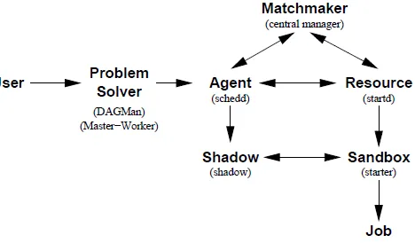
project [6]. Figure 2-1shows the architecture of the Condor and Condor-G in the Grid

(16)

5

Figure 2-1 Condor in the Grid (Figure 1 from [6])

Condor-G does not support all the features of GRAM, otherwise it would have become

complex and unusable [6].

2.1.2.2 Kernel and Condor Pool

Condor-G can be used in Grids for providing both the reliable submission and job

management service. The kernel of Condor-G performs the fundamental operations of

scheduling. The whole process is shown below:

When a job is sent by a user to an agent, the agent stores the job information in the

shadow.

1. Both the agent (A) and the resource (R) are in contact with the matchmaker (M).

(17)

6

3. The agent contacts the resource and validates the information about the resource,

and the agent sends the job to the resource for execution.

Figure 2-2 shows the whole scheduling process. In the figure, the sandbox provides the

resource to prevent mischief by other jobs. The process is executed in the Condor pool,

shown in Figure 2-3.

Figure 2-2 Scheduling Process (Figure 2 from [6])

Figure 2-3 Condor Pool (Figure 3 from [6]) 2.1.2.3 Gateway Flocking

Each condor pool may have a Gateway (G) for communication with other condor pools.

(18)

7

have a resource, which matches the requirements of the job, the Matchmaker (M) of the

condor pool A can go to a resource in another condor pool though the gateway of pool A. This process is called “Gateway Flocking”. Figure 2-4 shows the case of two condor

pools A and B. The matchmaker in pool A finds that none of the resources in pool A

matches the requirements of the job, submitted by agent A. So the matchmaker sends the

job requirements out through the gateway. The matchmaker in condor pool B finds that a

Resource R in condor pool B matches the requirements of the job, submitted by the agent

A in condor pool A.

Figure 2-4 Gateway Flocking (Figure 4 from [6])

2.1.2.4 Direct Flocking

Gateway Flocking supports communicating at the organizational level, while direct

flocking permits an individual user to join multiple communities. Instead of

communicating through the gateways, in direct flocking, an agent (A) reports itself to

(19)

8

Figure 2-5 Direct Flocking (Figure 6 from [6])

2.1.2.5 Scheduling through Foreign Batch Queues

When an agent receives a large number of jobs, it may execute the jobs through foreign

batch queues. This service is provided by Condor-G.

Figure 2-6 shows an example of scheduling of two jobs through foreign batch queues in

two different condor pools:

Figure 2-6 Scheduling through Foreign Batch Queues (Figure 7 of [6])

2.1.2.6 Gliding in

Thain et al. [6] state the following disadvantage of the Condor-G system:

 GRAM couples resource allocation and job execution, so that the agent must

direct a particular job to a particular queue. Furthermore, the queue-based system

(20)

9

To solve the problem, Thain et al. [6] used “gliding in” technique. The 3-step process

is explained through Figures 2-7, 2-8 and 2-9:

 Step 1: A Condor-G agent (A) submits the jobs, received by it, to two foreign

batch queues via GRAM, shown in Figure 2-7.

Figure 2-7 (Figure 8a from [6])

 Step 2: The resources form a personal condor pool with the user's personal

matchmaker, shown in Figure 2-8.

Figure 2-8 (Figure 8b from [6])

 Step 3: The agent gets the jobs executed through the resources in the personal

(21)

10

Figure 2-9 (Figure 8c from [6])

2.1.3 GridWay

Huedo et al. in [7] state that GridWay Framework is a tool that hides the complexity and

dynamicity of Grid from developers and users, allowing the solution of large

computational problems in a Grid environment by adapting the scheduling and execution

of jobs to the changes in Grid conditions and in the demands from application. The Local

Resource Management (LRM) system is the generic denomination for the cluster

component which manages the execution of user applications [8]. GridWay is a Local

Resource Management (LRM) like environment for submitting, monitoring, and

controlling jobs [11]. In GridWay Framework, a transfer queue is used for

communicating jobs from the Local Resource Management (LRM) system to the gridway

meta-schedulers [11]. When jobs are submitted to the system, they are put into the

transfer queue, and all the operations, such as start executing a job, terminating or

suspending a running job, or resuming a job, are all executed through the queue, shown in

Figure 2-10. It is concluded in [7] that GridWay provides adaptive scheduling and

(22)

11

Figure 2-10 Transfer Queue in Gridway

2.2 Local Search Based Scheduling

The scheduling problem is recognized as a NP-complete problem [12], [13]. Various

local search procedures have been developed for solving computational optimization.

Local search can be used on problems that can be formulated as finding a solution

maximizing a criterion among a number of candidate solutions. Local search algorithms

move from solution to solution in the space of candidate solutions (the search space)

until a solution deemed optimal is found or a time bound is elapsed.

Local search algorithms can be used to solve the distributed scheduling problems: Given

a set of distributed resources and jobs, scheduling is the process of allocating the jobs to

the compatible resources. The objective of scheduling is to satisfy both the QoS of the

users and the usage of the resources, and they are also used as the evaluation of the

(23)

12

application of the local search algorithm to the distributed scheduling are shown in Table

2-1:

Local Search Algorithm Distributed Scheduling Objective Finding a solution maximizing a

criterion among a number of candidate solutions.

Finding a schedule minimizing the makespan, number of delayed jobs, total tardiness, etc.

Solution A new solution is generated for each move.

A new schedule is generated for each one or several jobs arrival. Termination A solution deemed optimal is

found; A time bound is elapsed; The best solution found by the algorithm has not been improved in a given number of steps, etc.

A schedule deemed optimal is found; A time bound is elapsed; The best solution found by the algorithm has not been improved in a given number of steps, etc

Feature A deemed optimal solution (not

global optimal solution) can be found

A deemed optimal schedule (not global optimal schedule) can be found

Table 2-1 How to Apply Local Search Algorithm in Scheduling Problems

Most local search based scheduling algorithms use heuristics [4]. The heuristic

algorithms, such as Tabu Search (TS), Genetic Algorithm (GA), Simulated Annealing

(SA), and Ant Colony Optimization (ACO), are considered to be a good way to find a

local optimum solution in the search space [14].

Kousalya.K and Balasubramanie.P [14] showed the main strategy of Ant Colony

Optimization (ACO), while Abraham et al. [15] give a brief introduction Tabu Search

(TS), Genetic Algorithm (GA) and Simulated Annealing (SA).

2.2.1 Ant Colony Optimization

The Ant Colony Optimization (ACO) is a probabilistic technique for solving

computational problems. In Ant Colony Optimization (ACO), the ants try to build a

feasible solution to apply the stochastic decision policy repeatedly [14]. If one ant finds a

(24)

13

ants are more likely to follow that path, and positive feedback eventually leads all the

ants following a single path.

Kousalya.K and Balasubramanie.P [14], [16] use ACO to allocate a set of independent

jobs to a number of distributed resources. The objective is to obtain a schedule with a

minimum value of makespan. Three important values: pheromone (τij), the attractive of

the move as computed by some heuristic information (ηij), and the completion time of ith

job on the jth machine (CTij) are defined. The value of τij indicates a prior desirability of the current move, while ηij indicates how profiTable it has been in the past to make that

particular move [14]. The value Pij decides which job to be run, and which machine is

used to execute that job. Pijrepresents the probrability to move from a state i to a state j,

and is calculated by the formula Pij =

τ η

τ η . The proposed algorithm starts only if

there are some tasks which are not scheduled. The authors of [14] propose the use of two

algorithms. The value of pheromone evaporation ρ initialized to 0.05, while the pheromone deposit τ0 is set to 0.01. The number of ants is set to 2.

Algorithm 1 aims to schedule the jobs which are in the set of unscheduled job list, while

the local search algorithm is shown in Algorithm 2 for further optimization. The pseudo

(25)

14

Table 2-2 Algorithmic Frame for an Ant Algorithm (Algorithm 1 from [14])

Algorithm 1 can be concluded as the following 5 basic steps shown in Table 2-3, where

the first three steps are done by each ant, and the 4th and the 5th step are performed by the whole system:

Table 2-3 Ant Algorithm Applied in Scheduling Algorithm 1 Algorithmic frame for a Ant Algorithm:

For each Ant do

Randomly select Taskiand resourcej

Add (Taski, resourcej , free[j], free[j]+ETij) to the output list.

Remove the Taskifrom the unscheduled list to scheduled list

For each Taskiin the unscheduled list do

Calculate the heuristic information (ηij), where

A minimization function F and the heuristic information ηij is used to find out the best resource:

F = max(free(j)), and ηij = 1/ free(j)

Find out the current pheromone trail value (τij)

Update the pheromone trail matrix where,

τij = ρτij + Δτij

Calculate the Probability matrix where,

Pij =

Find out the highest value of Pijand add (Taski, resourcej , free[j],

free[j]+ETij) to the output list.

Remove the Taskifrom the unscheduled list

Modify the resource free time

free[j] = free[j] + ETij

done

Find out the best feasible solution by analyzing of all the ants scheduling list done

Step 1: Each ant randomly select job i from the set of tasks and resource j from the set of resources.

Step 2: Once a job is selected and scheduled, Task i is removed from the unscheduled list to the scheduled list.

Step 3: For each ant, in each iteration of Task i in the unscheduled list, calculate and find out the highest value (best solution) of Pij.

Here, each ant generates a list of solutions, we store the best solution from each list into set Sl, and then we select the best solution from Sl:

Step 4: Find out the best feasible solution from the scheduling list of all the ants.

(26)

15

After the solutions generated from Algorithm 1, there may have some „problem‟

resources that performs bad. The authors in [14] try to reduce the makespan using local

search techniques. The neighborhood is a solution of single transfer of a job from the

problem resource to any other resource [14], so that a new better solution may be

generated. This is shown in Algorithm 2, and some values are defined and initialized as:

 S:Current solution, initialized as (Taski, resourcej, free[j], free[j]+ETij) which is

generated from Algorithm 1.

 s‟: New generated solution (initialized to NULL).

The pseudo code of Algorithm 2 is shown in Table 2-4:

Table 2-4 Algorithmic Frame for a Local Search Algorithm (Algorithm 2 from [14])

Algorithm 2 can be concluded as the following 2 basic steps shown in Table 2-5: create a

set of neighbors of S, and find out the better solutions from the set of neighbors:

Table 2-5 Local Search Algorithm

Step 1: Create a set of neighbors of S, calculate the value of neighbor s‟. (The value of S and s‟ is evaluated by Pij.)

Step 2: If s‟ is better than S, then S=s‟. (A better solution is found)

Algorithm 2 Algorithmic frame for a local search algorithm:

Repeat until s‟ <> S

Find out the problem resource‟s and problem resource‟s problem job

Create neighbor of S(s‟) to transfer the problem job to some other resource

If s‟ is better quality than S then S = s‟

(27)

16

As a result, ACO is used in scheduling problem, and the experiment results in [14] shows

that using ACO algorithm can achieve better resource utilization and better scheduling.

2.2.2 Tabu Search

Tabu Search (TA) is a meta-strategy to solve local optimality and has become an

optimization approach that is used in many fields [15]. Tabu Search explores a set of problem solutions, repeatedly moves from one solution S to another solution S‟ in the

neighborhood N(S) of S, to find a local optimal evaluated by some objective functions

[15].

A template for simple Tabu Search [17] is shown in Table 2-6:

Table 2-6 Template for Simple Tabu Search (Simple Tabu Search in [17]) Notation:

 S: the current solution

 S*: the best-known solution

 f*: values of S*

 N(S): the neighborhood of S

 N‟(S): the “admissible” subset of N(S) (i.e. non-tabu or allowed by aspiration)

 T: tabu list

Initialization:

Choose (construct) an initial solution S0.

Set S: = S0, f*:=f(S0), S*:=S0, T:=ø Search:

While termination criterion not satisfied do

 Select S in argmin[(f(S‟));

S‟ N‟(S)

 If f(S) < f*, then set f*:=f(S), S*:=S;

 Record tabu for the current move in T (delete oldest entry if necessary);

Endwhile

(28)

17

Klusacek et al. [18] applied Tabu Search (TS) for dynamic arrived distributed job

scheduling problem. Rasooli [19] used Tabu Search based algorithm to allocate the

independent jobs to the distributed resources.

The Tabu Search optimization stated in [19] aims to minimize both the flowtime (the

total running time of all the jobs) and makespan (the maximum time that a job used) of

the whole process. According to the algorithm of scheduling in [19], the distributed jobs

are first, based on their deadline in ascending order, allocated to the resources, and

waiting for their execution in a set of queues. Before executing, Tabu Search

optimization is applied, that the jobs may be allocated to another position of the queues.

Once a job is moved to another position in the queue, the flowtime and the total

makespan are changed, and can be calculated by the scheduler in the system.

The Tabu Search Optimization applied in [19] can be described as the following 6 steps:

1. Select the resource with the highest expected flowtime/makespan.

2. Transfer the job which has the maximum completion time to other resources.

3. If a job is moved onto machines with smaller flowtime/makespan, the move is

accepted.

4. Once the job is moved, it is placed into the Tabu-list to prevent cyclic moves.

5. Once the machine is selected, it is placed into the Tabu-list to prevent cyclic

selection.

(29)

18

The experimental results in [19] show that using Tabu Search optimization can improve

the flowtime and makespan of the distributed job scheduling problems.

A scheduling problem solved using Tabu Search is shown in Section 2.3.3.

2.2.3 Simulated Annealing

Simulated Annealing (SA) is another heuristic that searches through the neighborhood of

an initial state to find a local optimum solution [15]. SA avoids getting trapped within a

local minimum [15]. At the beginning of the algorithm, the control parameters, T

(temperature), p (probability), and f (objective function) are set to an initial state. The

value T is reduced by a specific rate in each move, and once it is reduced to a specific

small value (set by the user), SA is terminated, and the solution is found.

Fidanova in [20] applied a SA-based algorithm to solve the scheduling problem. The

objective is to schedule all the incoming applications (jobs) to the available distributed

resources [20], and minimize the makespan for the complete schedule. The jobs are

distributed and independent, while the resources may be either homogeneous or

heterogeneous.

The author in [20] introduced three important variables: The completion time of job i on

machine j (CTij), the function free(j), and the starting time of job i (bi). The value of bi

indicates the starting time of job i on machine j, where machine j would have finished the

previously assigned jobs. The value of CTij is defined as the wall-clock time at which

machine j completes job i, and it is calculated according to the formula CTij = bi + ETij,

(30)

19

no load before the allocation of job i, bi = 0. Funtion free(j) indicates the time that

machine j is free, that is, the value of bi is decided by free(j).

The whole algorithm can be described as the following 5 steps:

 Generate the initial feasible solution S

As we mentioned, the objective is to schedule all the incoming applications (jobs) to the

available distributed resources, so the solution of each allocation is represented by the

triples (job, machine, starting time). For example, if one solution is written as (ji, mj, bi),

then it means job i is executed on machine j starting at time bi. The set of solutions can be

represented as a matrix M with three columns, the first column represents the jobs, the

second represents the machines to execute the job in the same row, and the third

represents the corresponding starting times. Each row of matrix M represents a solution.

S represents the set of the solutions (rows) of M. The author in [20] used a greedy

heuristic to create the initial solution: the first job executed on the first free machine j

with the minimal value of free(j), and the same method is used for the second job in the

set and so on.

 Initialize the Cooling Parameters

The author [20] has chosen the initial value of the temperature parameter T as 8 and the

cooling rate F as 0.9.

 Generate the neighbors and select the solutions from S

(31)

20

times and the free(j) functions are changed. If a better solution is generated from S‟, we

replace this new solution as the current best solution. This swapping step is repeated

according to the termination criterion, which is shown in the next two steps.

 Update the Temperature Parameters

The temperature parameter T is updated according to the formula Tk = F*Tk, where k = 1,

2, …

 Termination of the Solution (Termination Criterion)

The whole process is terminated if the value of T is updated less than a specific small

value Ѳ, (where 0< Ѳ <1).

The experimental results in [20] show that using SA algorithm can obtain good load

balancing of the machines and achieve a good performance

2.2.4 Genetic Algorithm

Genetic Algorithm (GA) can be used to solve optimization problems based on the genetic

process of biological organisms [15].

GA has four basic processes:

 Initialization: Randomly generate the initial population.

 Selection: A proportion of existing population is selected to breed a new

generation.

 Reproduction: Generate a second generation population through genetic operators:

(32)

21

 Termination: Terminate the process when the condition for termination is

reached.

Aggarwal.M et al. [13] applied Genetic Algorithm to “obtain the best schedule for

mapping of tasks to compute-nodes”. In this paper, the assumption is that the grid

workload may consist of multiple jobs, and each job is represented by a Directed Acyclic

Graph (DAG). In [21], Martino and Mililotti applied Genetic Algorithm to solve the

problem of “allocating a set of distributed jobs to a set of interconnected computing nodes”. Fissgus [22] applied Genetic Algorithm to solve the problem of “scheduling of

mixed task and data parallel modules comprising computation and communication operations” [22].

Abraham et al. [15] use Genetic Algorithm to allocate Jn (n=1, 2… N) independent user

jobs to Rm (m=1, 2, … M) heterogeneous resources, and to minimize the makespan, and

flowtime. The authors in [13] introduced an important variable: The completion time. It

is the time, when the last job j finishes processing (Cj). The makespan in [15] is defined

as Cmax = max {Cj, j = 1, …, N}, and flowtime as . To formulate the algorithm,

the authors of [15] also proposed 3 job lists and 3 resource lists:

(33)

22

Table 2-7 shows the pseudo code of GA approach for job scheduling applied in [15]:

Table 2-7 GA Approach for Job Scheduling on the Grid (GA Approach in [15]) 1. If the grid is active and (Jlist1=0) and no new jobs have been submitted, wait for new jobs to be submitted. Update Rlist1 and Jlist1.

2. If (Rlist1=0), wait until resources are available. If Jlist1>0, update Jlist2. If Jlist2 < Rlist1 (available resources) allocate the jobs on a first-come-first-serve basis and if possible allocate the longest job J on the fastest resource M according to the LJFR heuristic. If Jlist1 > Rlist1, job allocation is to be made by following the heuristic algorithm detailed below. Take jobs and available resources from Jlist2 and Rlist3.

3. At t =0; generate an initial population with P chromosomes Popi(t), encoding the schedules. Feasibility

of each chromosome is to be checked and makespan for each schedule represented by the chromosome is to be calculated. In certain cases, illegal offspring‟s (duplicated jobs, missing jobs, jobs outside the list) are generated due to genetic operators that require to be repaired immediately to ensure that each job appears only once in the sequence.

4. Begin GA loop

While (until the specified fitness value is achieved) do;

a. For each chromosome (i=1 to P), first allocate the jobs to the available resources based on the LJFM heuristic and once a resource is free (due to job completion), a job is allocated based on the SJFM heuristic. There after LJFR – SJFR heuristic is applied alternatively after completion of every job. Calculate the make span and total flowtime for the generated schedule. Also calculate fitness value of each chromosome, Fitnessi=FitPopi(t);

b. For (i=1 to P), Create new population NewPopi(t+1) which is choosen randomly based on the fitness value of each chromosome Popj(t) in the current population Pop(t). The probability for selection a

chromosome for the next generation may be defined as pj=

or according to the selection

strategy adopted;

c. Apply crossover operator on the population according to the probability selected, Crospop(t+1) = recombined chromosomes of the population NewPopi(t+1);

d. Apply mutation operator on the population according to the probability selected, MutPop(t+1)=mutated population CrosPop(t+1).

5. Evaluate fitness of each individual and when the Fitnessihas reached the required value end loop.

6. Check the feasibility of the generated schedule with respect to resource availability and user specified requirements. Then allocate the jobs to the resources and update Jlist2, JList3, RList2 and Rlist3. Un-allocated jobs (infeasible schedules or resource non-availability) shall be transferred to JList1 for re-scheduling or dealt with separately.

(34)

23

The basic steps of Genetic Algorithm: Initialization, Selection, Reproduction, and

Termination applied in the GA approach for job scheduling on the Grid in [15] are shown

in Table 2-8:

Table 2-8 Basic Steps of GA Approach

2.2.5 Hybrid Heuristic Algorithms

Some researchers have proposed hybrid heuristic algorithms. In [23], a hybridization of

Genetic Algorithms (GAs) and Tabu Search (TS) for scheduling independent tasks in

computational grids has been presented. In [24], an evolutionary hybrid scheduling

algorithm is proposed. Benedict et al. [24] state that Niched Pareto Genetic Algorithm

(NPGA) with Simulated Annealing (SA) works better than other heuristics, which they

have tested.

Abraham et al. [15] have evaluated scheduling systems based on GA, TS and SA. The

authors [15] claim that the hybridization of GA and SA algorithm provides a better Initialization: Randomly generate the initial population

Selection: Select the new population according to pj=

or the selection strategy adopted;

Reproduction:

 Crossover: Apply crossover operator on the population according to the probability selected, Crossop(t+1) = recombined chromosomes of the population NewPopi(t+1);

 Mutation: Apply mutation operator on the population according to the probability selected,

MutPop(t+1)=mutated population CrosPop(t+1).

(35)

24

convergence, while a hybrid GA and TS algorithm improves the search efficiency as

compared to a scheduler, which uses GA only.

Abraham et al. [15] proposed hybrids GA-SA approach for job scheduling in Grids.

Some steps of the hybrid GA-SA approach are the same as the GA approach stated in

section 2.2.4.

Table 2-9 shows the pseudo code of hybrid GA-SA approach in [15]:

Table 2-9 GA-SA Approach for Job Scheduling in Grid (GA-SA Approach in [15])

The GA-SA approach is different from GA approach applied for job scheduling on the

Grid in [15]. Instead of the reproduction step used in GA approach, GA-SA applies two

basic steps of SA: cooling loop and reheating loop, which help to find a better schedule. 1 and 2 are the same as used in GA.

3 Generate an initial population of P schedule vectors and for i =1 to P, initialize the ith threshold,

Th(i), with the energy of the ith configuration. For each schedule (i=1 to P), first allocate the jobs to

the available resources based on the LJFM heuristic and once a resource is free (due to job completion), a job is allocated based on the SJFM heuristic. There after LJFR – SJFR heuristic is applied alternatively after completion of every job.

4 Begin the cooling loop

Energy bank (EB) is set to zero and for i = 1 to N randomly mutate the ith schedule vector. Compute the Energy (E) of the resulting mutant schedule vector.

If E Th(i) , then the old configuration is restored.

If E Th(i) , then the energy difference (Th(i) –E) is incremented to the Energy Bank (EB) =

EB+Th(i) –E. Replace old configuration with the successful mutant End cooling loop.

5 Begin reheating loop.

 Compute reheating increment eb= , for i = 1 to N. (Ti(k) = cooling constant).

 Add the computed increment to each threshold of the schedule vector.

End reheating loop.

6 Go to step 4 and continue the annealing and reheating process until an optimum schedule vector is found.

(36)

25

If an acceptable optimum schedule vector is found in the cooling and reheating process,

the whole process is terminated.

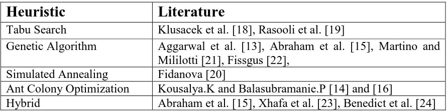
Heuristic

Literature

Tabu Search Klusacek et al. [18], Rasooli et al. [19]

Genetic Algorithm Aggarwal et al. [13], Abraham et al. [15], Martino and Mililotti [21], Fissgus [22],

Simulated Annealing Fidanova [20]

Ant Colony Optimization Kousalya.K and Balasubramanie.P [14] and [16]

Hybrid Abraham et al. [15], Xhafa et al. [23], Benedict et al. [24]

Table 2-10 Literature on the Use of Local Search Algorithms to Develop Grid Scheduler

2.3 Schedule Based Scheduling

Schedule based scheduling methods allow precise mapping of jobs onto resources in a

dynamic environment [4]. The advanced Grid resource management system GORBA

[25], as well as CCS [26] use schedule based policies to schedule jobs or workflows.

Furthermore, in [6] and [25], heuristic algorithms are also applied for their further

optimization.

2.3.1 GORBA

GORBA (Global Optimizing Resource Broker and Allocator) uses simple polices to

create the schedule, and applies a heuristic algorithm as its optimization method. Suß et al.

[25] state that the applications in GORBA are represented as workflows, while the

resource broker is the component to form and calculate the schedule as well as planning

for the future resource deployment. In GORBA, each work node is managed by the

(37)

26

GORBA for optimizing the schedules. HyGLEAM is a combination of the Evolutionary

Algorithm GLEAM (General Learning Evolutionary Algorithm and Method) and local

search algorithms [27]. Jakob et al. [27] state that GLEAM algorithm consists of the

Evolution Strategy and real-coded Genetic Algorithms with data structuring concepts.

The local search algorithms used by HyGLEAM are the Rosenbrock algorithm [28] and

the Complex method [29].

Stucky et al. [30] state that if time constraint exists, only one heuristic is deployed. In

addition, due to the re-schedule strategy, it is quite time consuming for the large number

of jobs [30]. In GORBA, an application and resource management system is embedded

between two interfaces:

 The Grid Application Interface (GAI) to users and to administrators [30]

 Interfaces to third-party grid middleware, such as Globus service [30]

Grid Application Interface (GAI) mediates between the application and resource

management system. GORBA uses a third-party middleware layer to get up-to-date

information of the resources [30]. Currently, GORBA uses Globus service as its

third-party middleware, but it is planned to be flexible in deploying third-third-party software and

utilize UNICORE alternatively [25].

Figure 2-11 shows the architecture of the GORBA system in Grid, and the coarse

(38)

27

Figure 2-11 Architecture of GORBA in Grid (a) and the coarse architecture of GORBA

(b) (Figure 1 from [30])

2.3.2 CCS

Hovestadt et al. [26] state that advanced reservation and quality of service are needed to

be solved by co-allocation. It is hard for queuing approach based resource management

system to solve this problem. Instead, advanced reservations can be solved by planning

approach: assigning start times to each resource request, so that a complete schedule is

planned. CCS (Computing Center Software) [26] has been designed to provide “a uniform access interface” [31] for HPC users, and provide “a means for describing,

organizing, and managing high performance computing (HPC) systems” [26] for system

administrators.

A complete schedule about the future resource usage is computed and made available to

the users. First Come First Serve (FCFS), Shortest/Longest Job First (SJF/LJF) policies

(39)

28

of the schedule. CCS re-computes the schedule from scratch when a dynamic change

such as job arrival or machine failure appears [4].

Fig 2-12 shows the 5 components of (Computing Center Software) CCS

Figure 2-12 Architecture of CCS (Figure 3 from [26])

 The User Interface provides a single access point to one or more system via an

X-window or ASCII interface.

 The Access Manager (AM) manages the user interfaces and is responsible for

authentication, authorization, and accounting.

 The Planning Manager (PM) plans the user requests onto the machine.

 The Machine Manager (MM) provides an interface to machine specific features

like system partitioning, job controlling, etc.

 The Island Manager (IM) / Domain Manager (OM) provides name service and

watchdog facilities to keep the island/domain in a sTable condition.

Computing Center Software (CCS) provides mechanisms for the user-friendly system

(40)

29

a schedule based system in [4]. CCS is able to handle both advanced reservation and

quality of service [26], [31].

2.3.3 Earlier Gap, Earliest Deadline First and Tabu Search Optimization

Klusacek and Matyska [2] applied a schedule based method to handle the scheduling in

dynamic environment. Dynamic jobs arrival is simulated, and a Tabu Search optimization

is used for further optimizing the schedule.

Earlier Gap, Earliest Deadline First (EG-EDF), combined with Tabu Search Optimization

is a solution designed and applied by Klusacek and Matyska [2] to simulate and solve “the distributed large scale dynamic arrived jobs scheduling” problem. Earlier Gap,

Earliest Deadline First (EG-EDF) and Tabu Search Optimization are the two main parts

of the scheduling process. Earlier Gap, Earliest Deadline First (EG-EDF) add newly

arrived jobs to the schedule, while Tabu Search Optimization moves the jobs already

allocated in the schedule and make further optimization for the schedule. Earlier Gap,

Earliest Deadline First (EG-EDF) is applied for any time a new job arrives, while Tabu

Search Optimization is applied after every 10 jobs have arrived.

The authors [2] attempt to satisfy three objectives: Minimizing the total tardiness (the

total delayed time) of the jobs, the number of the delayed jobs, and the makespan (the

processing time from the first start of the first job execution to the end time of the last

execution) of the whole scheduling process.

(41)

30

Earlier Gap, Earliest Deadline First (EG-EDF) algorithm is applied for each newly

arrived job into the existing schedule of each resource. Once a new job arrives, the best

position for the job according to the current schedule is selected.

Gaps may be generated during the execution. A gap is considered to be the CPU idle (no

job is executing on some CPUs of some machines) of the machines during the execution.

A suitable gap for a job means the gap contains more CPUs than the job required. Figure

2-13 shows an example of a gap with 2 CPUs generated at time t0.

(42)

31

Figure 2-14 Earlier Gap, Earliest Deadline First

Figure 2-14 shows the main strategy of Earlier Gap, Earliest Deadline First (EG-EDF)

Algorithm. When a new job arrives, it follows the following policies:

1. Gap 1 to gap 11 represent the suitable gaps for new arriving job, and all of them are

candidate positions.

2. Generally, jobs on schedules of each machine are sorted according to their deadline.

The deadline of the new arrived job is assumed between the kth and the k+1th job on

each schedule. So, positions between k to k+1 of each schedule of machine are candidate

positions.

3. EG-EDF tries on all the candidate positions, evaluates and figures out which candidate

performs the best.

4. The scheduler search for all the candidate positions from the first machine to the last.

For each machine, it is searched from the earliest candidate position to the latest one.

(43)

32

6. The scheduler has all the information of the machines, schedules, and the jobs arrived.

7. The performance are evaluated by the three objectives: makespan, tardiness, and

number of delayed jobs by using AcceptanceCriterion().

The pseudo code of EG-EDF is listed in Table 2-11 and Table 2-12:

Table 2-11 Earliest Gap, Earlier Deadline First (EG-EDF from [2])

Table 2-12 Method AcceptanceCriterion() (AcceptanceCriterion() from [2]) Algorithm 1 Earliest Gap – Earlier Deadline First (job)

1: scheduleinitial := [mach sched1, .., mach schedm]; schedulenew := ; schedulebest := ; gap_found := false; k := 0;

2: fori := 0 to mdo

3: ifmachinei is suiTable to perform jobthen

4: if suiTable gap for job was found in schedulenew[i] then

5: gap_found := true; 6: schedulenew := scheduleinitial;

7: schedulenew[i] := place job into found gap in schedulenew[i]; (EG strategy)

8: else ifgap_found = false then

9: schedulenew := scheduleinitial;

10: k := index of the first jobk schedulenew[i] whose djobk > djob; (k is the

index of the first job with later deadline)

11: schedulenew[i] := insert job into schedulenew[i] between jobk−1 and jobk;

(EDF strategy) 12: end if

13: if AcceptanceCriterion(schedulebest, schedulenew) = true then

14: schedulebest := schedulenew;

15: end if

16: end if

17: end for

18: returnschedulebest

Algorithm 2 AcceptanceCriterion(schedulebest, schedulenew)

1: if schedulebest = ; then

2: return true; 3: end if

4: compute makespanbest and nondelayedbest according to schedulebest;

5: compute makespannew and nondelayednew according to schedulenew;

6: weightmakespan := (makespanbest − makespannew)/(makespanbest);

7: weightdeadline := (nondelayednew − nondelayedbest)/(nondelayedbest);

8: weight := weightmakespan + weightdeadline;

9: ifweight > 0.0 then

10: return true; 11: else

(44)

33 2.3.3.2 Tabu Search Optimization

Unlike Earliest Gap, Earlier Deadline First (EG-EDF), Tabu Search is applied to make

some further optimization for the jobs which are already allocated to the schedule of each

machine. Tabu Search Optimization is necessary, even if the jobs are currently allocated

to the best position by Earliest Gap, Earlier Deadline First (EG-EDF). EG_EDF

algorithm does not guarantee to generate the best solution, when more new jobs arrive.

Furthermore, once a job is allocated, even if a better solution were possible, EG_EDF

will not allow the jobs to be moved.

As we mentioned, EG-EDF algorithm is applied for every newly arrived job, while Tabu

Search algorithm is used for every 10 jobs arrived. Tabu Search is a local search based

heuristic algorithm. The maximum number of iterations of the Tabu Search manipulation

in [2] is set to 1000. During each iteration, only one job in the schedule is to be moved.

Before showing the Tabu Search Optimization, there are two concepts to introduce:

 Tabu Job

Tabu-Job is generated during the Tabu Search Optimization. TabuList is a list with

specific size. In the process of Tabu Search Optimization, once a job is moved, or put

back to the original position, it is put into the TabuList, and once a job is put into the

TabuList, it becomes a tabu-job. Once a job becomes a tabu-job, it is no longer a

candidate job that considered to be moved. Furthermore, sometimes the TabuList may be

full, and a new job is put into the TabuList. In this case, the job first put into the TabuList

(45)

34

For example, if there the size of TabuList is 5 and now we put the 6th job into the TabuList. In this case, the 1st job in the TabuList is no longer a Tabu-Job.

The number of Tabu-Job is initialized as 0.

 Machine Used

The jobs have allocated by EG-EDF are stored in the schedules of machines, waiting for

their executions or further moving by Tabu Search Optimization. In each iteration of

Tabu Search Optimization, only one job is considered to be moved. Before selecting the

jobs, the machine is selected in advance. If in some iteration, a machine may contain only

tabu-jobs in its schedule. In that case, this machine becomes a “Machine Used”, or a used

machine. Used machines are not considered to be a source to select.

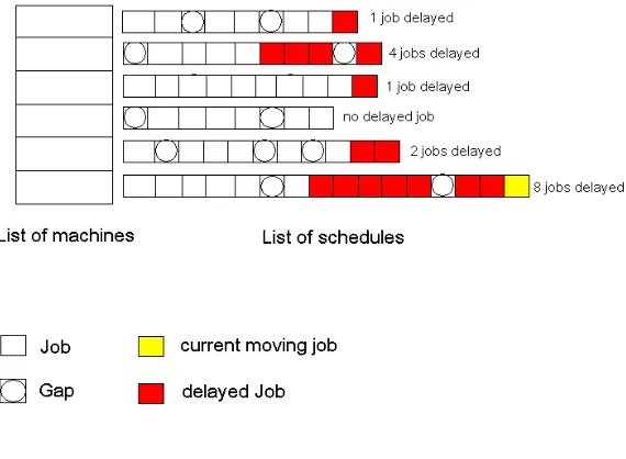
Figure 2-15 and 2-16 show the main strategy of Tabu Search Optimization. When every

10 jobs have arrived and when the jobs have been allocated to suitable machines by

EG-EDF, Tabu Search Optimization is applied and follows the following policies:

1. Before Tabu Search Optimization, all the machines and the jobs allocated in the

schedules by EG-EDF are not in the “Tabu Job” and “Machine_used” List.

1. The Scheduler knows which jobs have been delayed.

2. In each iteration, the job selected to be moved is the last “non-tabu job” in the schedule

of the “not used machine”with the highest number of delayed job.

3. Assume all gaps in Figure 2-15 are the suitable gaps for the job to be moved by Tabu

(46)

35

Figure 2-15 Tabu Search Optimization – Before Moving a Job

4. Tabu Search Optimization tries to move the job to the candidate positions, once a

better performance occurs, the current iteration terminates, and the job is moved. A new

iteration is started, shown in Figure 2-16.

(47)

36

5. If no better performance is found, the job is moved back to the original position and a

new iteration is started.

6. Once a new iteration starts, the job tested in the last iteration is set as a “tabu-job”,

shown in Figure 2-17.

Figure 2-17 Tabu Job

7. Once a machine contains only “tabu jobs”, it is set to a used machine, shown in Figure

2-18. And once all the machines are used machines, a new iteration is started, and all the

(48)

37

Figure 2-18 Machine Used

(49)

38

The pseudo code of Tabu Search Optimization is listed in Table 2-13 and Table 2-14:

Table 2-13 Tabu Search Optimization (Tabu Search from [2])

Table 2-14 Method MoveJob() (MoveJob() from [2]) Algorithm 3 Tabu Search (iterations)

1: schedulebest := [mach sched1, .., mach schedm]; schedulenew:= schedulebest; tabujobs:= ; machinesused:= ;

2: fori := 0 to iterationsdo

3: source := k such that: k (1..m), machinek machinesused, schedulenew[k] has highest number of

delayed jobs;

4: ifsource = null then

5: machinesused := ; (All machines were used – start a new round)

6: continue with new iteration; 7: end if

8: job := last job from schedulenew[source] such that: job tabujobs;

9: ifjob = nullthen

10: machinesused := machinesused machinesource; (No non-tabu job is available in schedulenew[source])

11: continue with new iteration; 12: end if

13: remove job from schedulenew[source];

14: if MoveJob(job, schedulebest, schedulenew) = false then

15: schedulenew := schedulebest; (returns job to the original position);

16: else

17: schedulebest := schedulenew; (updates the best so far found solution)

18: end if

19: tabujobs := tabujobs job; (and remove oldest item if tabujobs is full)

20: end for

21: returnschedulebest

Algorithm 4 MoveJob(job, schedulebest, schedulenew)

1: Sort the list of machines with their number of CPUs, if two machines have the same number CPUs, sort them according to

their speed; 2: forj := 0 to mdo

3: ifmachinej is suitable to perform job andsuiTable gap for job was found in schedulenew[j] then

4: schedulenew[j] := place job into found gap in schedulenew[j];

5: if AcceptanceCriterion(schedulebest, schedulenew) = true then

6: return true; 7: else

8: schedulenew[j] := schedulebest[j] (removes the proposed move);}

9: end if

10: end if

11: end for

(50)

39

3. Motivation and Model Formalization

3.1 Motivation

In Chapter 2, we mentioned the schedule based scheduling method EG-EDF and Tabu

Search Optimization. EG-EDF policy applied in [2] make use of resources by the

utilization of gap, and the centralized scheduler is responsible for the evaluation of the

performance of the whole system, such as makespan, tardiness, number of delayed jobs,

and resource utilization.

As we mentioned, Tabu Search Optimization [2] method is applied to further optimize

the performance after applying EG-EDF policy. However, it may generate some

shortcomings that influent the whole performance. As we mentioned in chapter 2, the

schedules are changed only according to the characteristics of the jobs waiting in the

schedule. Every 10 jobs arrive, the scheduler would make alternations on the schedules

according to the characteristics of those 10 jobs as well as the jobs former arrived but not

starting their executions. This leads to the randomization of the alternation of the

schedule, as well as the whole performance. Furthermore, it is impossible to guarantee

the completion time of each machine at the same time.

Figure 3-1 and 3-2 shows the schedule forms after applying EG-EDF and Tabu Search

(51)

40

Figure 3-1 List of Schedules

Figure 3-2 List of Completion Time

In Figure 3-1, the machines are sorted according to their speed of CPUs in descending

order. The lengths of jobs that each machine handles are random, so that the completion

time (shown in Figure 3-2) of each machine would also random, and it is impossible to

complete the executions of each machine at the same time.

To fix this shortcoming, we aim to figure out a new optimization method to complete the

execution of each machine at the same time. We allocate more lengths of jobs to the

machines which have higher speeds, and fewer lengths of jobs to the machines which have

slower speeds. The ideal schedules and completion times we aim to form are shown in

(52)

41

Figure 3-3 Objective List of Schedules

Figure 3-4 Objective List of Completion Times

3.2 Model Formalization

In this thesis, we attempt to solve the optimal scheduling problem in a dynamic model.

However we assume that the computational resources are a set of machines, which are

waiting for the arrival of a dynamic set of independent jobs. During the execution, once a

job arrives, it is allocated to an appropriate machine by using a well-defined policy.

Before introducing the algorithm, we describe some basic definitions.

 Release date, of a job represents the time of arrival of that job.

 Deadline of a job is the desired completion time of that job.

(53)

42

 The tardiness of job j is defined as the time interval between the actual completion

time and the deadline of the job j.

 Job j may require one or more CPUs for its execution. Let m be the number of

CPUs required by the job j during a particular interval of time after its release.

During this interval of time, let n be the number of free CPUs available with

resource i. Then job j can be executed on machine i provided n is greater than or

equal to m.

 The interval of time is time required to execute job j. It will depend upon the speed

of the machine i, and the length of job j.

Each machine in our work represents one resource, and contains multiple processors

(CPUs). All the CPUs within a machine are assumed to be identical. The machines have

the same allocation policy: It is not allowed to execute the same job on two or more

machines. Moreover, once a job is being executed, it is not moveable until its completion.

3.3 Evaluation Criteria

We use 4 criteria for evaluating the quality of the schedule:

 Makespan

 Number of delayed jobs

 Tardiness

(54)

43

3.4 Objectives

The two objectives of this thesis are:

1) Minimize the criteria: makespan, number of delayed job, tardiness, and machine

utilization;

Resource Characteristic Based Optimization for Grid Scheduling

Scholarship at UWindsor

Scholarship at UWindsor

Resource Characteristic Based Optimization for Grid Scheduling

Resource Characteristic Based Optimization for Grid Scheduling

Resource Characteristic Based Optimization for Grid

Scheduling

by

Peng Du

Abstract

Contents

List of Figures

List of Tables

1.

Introduction

2.

Related Works

Heuristic

Literature

3.

Motivation and Model Formalization