Volume 2009, Article ID 137451,20pages doi:10.1155/2009/137451
Research Article
Multipoint Singular Boundary-Value Problem for
Systems of Nonlinear Differential Equations
Jarom´ır Ba ˇstinec,
1Josef Dibl´ık,
1, 2and Zden ˇek ˇSmarda
11Department of Mathematics, Faculty of Electrical Engineering and Communication,
Brno University of Technology, Technick´a 8, 616 00 Brno, Czech Republic
2Department of Mathematics and Descriptive Geometry, Faculty of Civil Engineering,
Brno University of Technology, ˇZiˇzkova 17, 662 37 Brno, Czech Republic
Correspondence should be addressed to Josef Dibl´ık,[email protected]
Received 14 April 2009; Revised 9 July 2009; Accepted 16 August 2009
Recommended by Donal O’Regan
A singular Cauchy-Nicoletti problem for a system of nonlinear ordinary differential equations is considered. With the aid of combination of Wa ˙zewski’s topological method and Schauder’s principle, the theorem concerning the existence of a solution of this problemhaving the graph in a prescribed domainis proved.
Copyrightq2009 Jarom´ır Baˇstinec et al. This is an open access article distributed under the Creative Commons Attribution License, which permits unrestricted use, distribution, and reproduction in any medium, provided the original work is properly cited.
1. Introduction
In the present paper the following Cauchy-Nicoletti problem
yifi
x, y, i1, . . . , n, 1.1
yp
xpAp, yq
x±qAq, yr
xr−Ar,
p1, . . . , k; qk1, . . . , s; rs1, . . . , n
1.2
is considered, wherey y1, . . . , yn,x ∈ I a, banda x1 · · · xk < xk1 ≤ · · · ≤ xs < xs1 · · · xn b; Ai,i 1, . . . , nare real constants. DenoteIi I\ {xi},i 1, . . . , n
andJ ni1Ii.We will supposefi ∈ CΘi,R,i 1, . . . , nwhere the domainΘi ⊂ Ii×Rn
satisfying a relationΘi∩{xx∗}/∅for everyx∗∈Iiis more precisely specified inSection 2.
The continuity of the functionfiis not required at the pointxi,i 1, . . . , n.Solution of the
Definition 1.1. A vector-functionyx y1x, . . . , ynx ∈ CI,Rn with yi ∈ C1Ii,R,
i1, . . . , n,is said to be a solution of the problem1.1,1.2if it satisfies the system1.1on Jand if, moreover, conditions1.2hold.
Although singular boundary value problems were widely considered by using various methodssee, e.g.,1–11, the method used here is based on a different approach. Namely, it uses simultaneously the topological method of Wa ˙zewski and Schauder’s principle. Note that the method of Wa ˙zewski see, e.g., 12–14 was used for the investigation of various asymptotic and singular problems, for example, in3–6,11,12,15. For successful generalization of this to multipoint boundary-value problems, the basic obstacle must be overcome: the applying of topological method assumes that every intersection of so-called regular polyfacial set and the planex x∗ const,x∗ ∈ a, bis an open set in the space of dependent variables. Nature of the problems considered, as followed from problem1.1, 1.2does not permit straightforward generalization of this approach since the cross-section by the planexxi,i1, . . . , nis not an open set in the spacey. The above mentioned obstacle
is overcome in the present paper by connecting the topological method and the fixed point theorem.
Let us explain the main idea of this approach. Each equation of the system1.1is considered separatelyas a scalar equationunder the supposition that nondiagonal variables are changed by functions taken from a prescribed set M of vector functions. For every scalar equationtogether with the corresponding Cauchy initial condition which is subtracted from1.2it is, with the aid of Wa ˙zewski’s method and qualitative properties of solutions of differential equations, showed that there exists its solution having the same properties which were supposed for the corresponding coordinate of vector functions from M. In this way an operator T is defined. For verification of conditions of Schauder’s principle namely, the continuity of operatorT, Wa ˙zewski’s method is used again. Stationary point of operatorTdefines a solution of the problem1.1,1.2. The paper is organized as follows. InSection 2the main result is formulated. Illustrative examples are contained inSection 3. Auxiliary results are stated in Section 4. In Section 5 we prove results concerning scalar singular problems and the last section contains the proof of the main result.
2. Existence of Solutions of the Problem
1.1
,
1.2
Letαi, βi∈C1I,R,i1,2, . . . , nbe functions satisfyingαixi βixi Aiandαix< βix
onIi. Define
Ω x, y1, . . . , yn
:x∈I, αix≤yi≤βix, i1, . . . , n
, Ωi
x, y1, . . . , yn
:x∈Ii,
x, y1, . . . , yn
∈Ω. 2.1
Let us suppose that there exists a domainΘi,i 1,2. . . , nsuch thatΩi ⊂Θi ⊂Ii×Rn; cross
sectionSix {x, y ∈ Θi}is an open set for every fixedx ∈Iiandfi ∈ CΘi,R. These
assumptions are supposed in the sequel. Define, moreover,
Γi
x, yi1, . . . , yin−1
:x∈Ii, {i1, . . . , in−1}{1, . . . , n} \ {i},
αsx≤ys≤βsx, si1, . . . , in−1
,
Fi
x, y≡fi
x, y−yi, i1, . . . , n.
Result of the paper is given in the following theorem.
Theorem 2.1. Assume that
n
j1
Mijxyj−zj≤fi
x, y−fix, z≤ n
j1
Nijxyj−zj 2.3
for everyx, y1, . . . , yn,x, z1, . . . , zn∈Ωiwithyi> ziwhereMijx,Nijx, i, j1, . . . , n, are
continuous onIifunctions, such that for a constantξ >0
|Miix|> ξ n
j1,j /i
Mijx, |Niix|> ξ n j1,j /i
Nijx. 2.4
Let, moreover,
Fix, yyiαix·Fix, yyiβix<0,
signMiix signNiix signFix, yyiβix,
2.5
if x, y1, . . . , yi−1, yi1, . . . , yn ∈ Γi, i 1, . . . , n. Then there exists at least one solution yx
y1x, . . . , ynxof the problem1.1,1.2such that onIi, i1, . . . , n:
αix< yix< βix. 2.6
Remark 2.2. In the formulation of the problem1.1,1.2the inequalitiesxk < xk1andxs <
xs1 were supposed. Analyzing the method of proof ofTheorem 2.1we conclude that the
result remains valid in the cases whenxk≤xk1andxs ≤xs1too. This means, for example,
that a singular Cauchy problem
yifi
x, y, yi
x1Ai, i1, . . . , n 2.7
is a partial case of given result as well as a two-point boundary-value problem:
yifi
x, y, i1, . . . , n
yp
x1Ap, p1, . . . , k, yr
xn−Ar, r k1, . . . , n.
2.8
Remark 2.3. In 9 a technique based on Kneser’s theorem is introduced to extend the topological method of Wa ˙zewski for Carath´eodory systems. It has, for example, been used to study the asymptotic behavior of the solutions of a perturbed linear system:
˙
where then×nmatricesAdiagonalandBare locally integrable,g ∈Carloct0,∞×Cn,
and the solutions are unique with respect to their initial values. The existence of solutions xp xp1, xp2, . . . , xpn,p1,2, . . . , nsuch that for anyi /p
lim
t→ ∞
xpit
xppt
0 2.10
is studied. This is accomplished with the above-mentioned extension of the topological retract method for Carath´edory systems which can be applied due to the construction of a suitable regular polyfacial sets. This technique makes it possible to extend the results initially proved by Wa ˙zewski’s methodfor ordinary differential equations with continuous right-hand sides to Carath´edory systems. Similar method has, for example, been used in a recent paper6
where the technique developed in9is utilized. Along these lines, we can analyse our result in terms of its possible extension to systems1.1with Carath´eodory right-hand sides. Since the Lipschitz-type condition2.3is necessary in the proof ofTheorem 2.1for verifying the continuity of the operatorT, it cannot be omitted. Therefore, our result seems to be extendable for Carath´eodory systems1.1if the uniqueness of the solutions is ensured with respect to their initial valuessave at singular points.
3. Examples
Let us consider two illustrative nonlinear systems. The first one has a linear part which determines the existence of the solution of the problem considered. The second one is a perturbation of a system for which we know analytic solution of singular problem.
Example 3.1. Let us consider a singular problem:
y1 2y1 x −
xy2 31
10 ,
y2 y2 x−1/22 −
y1y31
20x−1/2,
y3 − 3y3 1−x
1−xy2 21
10 ,
y10 0, y2
1 2±
0, y3
1−0.
3.1
For this problem all conditions ofTheorem 2.1are valid for
α1x 0, β1x 3x,
α2x ⎧ ⎪ ⎪ ⎪ ⎨ ⎪ ⎪ ⎪ ⎩
3
x− 1 2
, if x∈
0,1 2
,
0, if x∈
1 2,1
β2x ⎧ ⎪ ⎪ ⎪ ⎨ ⎪ ⎪ ⎪ ⎩
0, ifx∈
0,1 2
,
3
x−1 2
, ifx∈
1 2,1
,
α3x 0, β3x 31−x2
3.2
and, for example, forξ1,M11x N11x 2/x,M12x N12x M31x N31x 0, M13x −N13x −3x1−x2/5,M21x M23x −N21x −N23x −1/20|x−
1/2|,M22x N22x 1/x−1/22, M32x −N32x −|x−1/2|, andM33x −N33x −3/1−x.Consequently, there is at least one solution to this problemyx y1x, y2x, y3xsuch that
0< y1x<3x forx∈0,1,
min
3
x−1 2
; 0
< y2x<max
0; 3
x−1 2
forx∈
0,1 2
∪
1 2,1
,
0< y3x<31−x2 forx∈0,1.
3.3
Example 3.2. Let us consider a singular problem:
y1 2 x3y
2
1εx2y22,
y2 3
x−1/24y
2 2ε
x−1 2
3 y23,
y3 −2 1−x3y
2
3ε1−x 2y2
1,
y10 0, y2
1 2±
0, y3
1−0,
3.4
whereεis a real constant,|ε|<0.01. For this problem all conditions ofTheorem 2.1are valid, for example, for
α1x x2−0.1x3, β1x x20.1x3,
α2x
x−1 2
3 −0.1
x−1 2
4
, β2x
x−1 2
3 0.1
x− 1 2
4 ,
α3x 1−x2−0.11−x3, β3x 1−x20.11−x3
3.5
and forξ 1,M11x 2/x,M12x M31x −N12x −N31x −M23x N23x −0.1,N11x 6/x,M13x N13x M21x N21x M32x N32x 0,M22x −12/1/2−x if x <1/2, N22x −5/1/2−x if x <1/2, M22x 3/x−1/2 if x >
Consequently, there is at least one solution to this problemyx y1x, y2x, y3xsuch
that
x2−0.1x3 < y
1x< x20.1x3 forx∈0,1,
x− 1 2
3 −0.1
x−1 2
4
< y2x<
x−1 2
3 0.1
x−1 2
4
forx∈0,1\
1 2
,
1−x2−0.11−x3 < y3x<1−x20.11−x3 forx∈0,1.
3.6
Ifε0, then the considered system turns into system
y1 2 x3y
2
1, y2
3 x−1/24y
2
2, y3 −2 1−x3y
2
3, 3.7
having solution
y1x2, y2
x−1 2
3
, y3 1−x2, 3.8
which satisfies3.4.
4. Preliminaries
In the sequel we will apply topological method of Wa ˙zewskisee, e.g.,12–14. Therefore we give a short summary of it. Let us consider the system of ordinary differential equations
ygx, y 4.1
with y ∈ Rn. Below, it will be assumed that the right-hand sides of the system 4.1are
continuous functions defined on an openx, y-setΩ∗⊂R×Rn.
Definition 4.1see12. An open subsetΩ0of the setΩ∗is called ann, p-subset ofΩ∗with
respect to the system4.1if the following conditions are satisfied.
1There exist continuously differentiable functionsni : Ω∗ → R, i 1, . . . , and
pj :Ω∗ → R, j 1, . . . , m; m >0 such that
Ω0x, y∈Ω∗:n
i
x, y<0, pj
x, y<0 ∀i, j. 4.2
2n˙αx, y < 0 holds for the derivatives of the functionsnαx, y,α 1, . . . , along
trajectories of the system4.1on the set
Nα
x, y∈Ω∗, nα
x, y0, ni
x, y≤0, pj
3p˙βx, y > 0 holds for the derivatives of the functions pβx, y,β 1, . . . , malong
trajectories of the system4.1on the set
Pβ
x, y∈Ω∗, pβ
x, y0, ni
x, y≤0, pj
x, y≤0∀iandj /β. 4.4
As usual, ifω⊂R×Rn, then intω, ∂ωandωdenote the interior, the boundary, and the closure
ofω, respectively.
Definition 4.2. The pointx0, y0∈Ω∗∩∂Ω0is called anegress pointoringress pointofΩ0with
respect to the system4.1if, for every fixed solution of the problemyx0 y0, there exists
anε >0 such thatx, yx∈Ω0forx
0−ε≤x < x0x0< x≤x0ε. An egress pointingress
point x0, y0ofΩ0is called astrict egress pointstrict ingress pointofΩ0ifx, yx/∈Ω0on
intervalx0< x≤x0ε1x0−ε1 ≤x < x0for anε1>0.
The set of all points of egressstrict egressis denoted byΩ0
e Ω0se. It is proved in12,
page 281, that when a setΩ0is ann, p-subset ofΩ∗thenΩ0 e≡Ω0se.
Theorem 4.3see12, page 282. LetΩ0 be somen, p-subset ofΩ∗ with respect to the system
4.1. LetSbe a nonempty compact subset ofΩ0∪Ω0
esuch that the setS∩Ω0eis not a retract ofSbut
is a retract ofΩ0
e. Then there is at least one pointx0, y0∈S∩Ω0such that the graph of a solution yxof the Cauchy problem yx0 y0 for4.1lies inΩ0 on its right-hand maximal interval of
existence.
5. Partial Singular Problems
At this part we are interested in existence of solutions of some auxiliary singular problems forone scalar equation. We consider two cases below with respect to the location of singular pointat the left end or at the right end of the interval considered.
5.1. Singular Point Coincides with the Left End of Interval
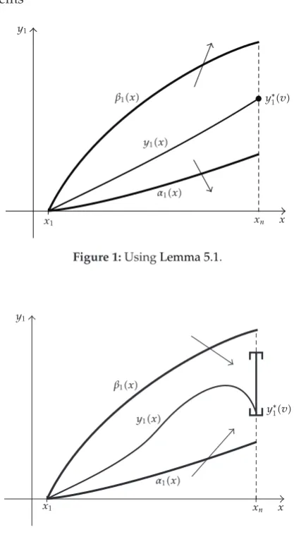
Consider the initial problem
yBx, y, 5.1
yu K, K∈R 5.2
on an intervalu, vwithu < v. By a solution of problem5.1,5.2on intervalu, vwe mean the function y ∈ Cu, v,R∩C1u, v,R which satisfies 5.1 on u, v and the
condition 5.2. Let functions λx, μx be continuously differentiable on u, v, λu μu Kandλx< μxonu, v. Denote
Let us suppose that there exists a domainΘ ⊂ u, v×R, such thatΘ ⊂ Θ and the cross sectionSx {x, y∈Θ}is an open set for everyx∈u, v. Define an auxiliary function
Hx, y≡Bx, y−y. 5.4
Lemma 5.1. Suppose that B ∈ CΘ, R satisfies the local Lipschitz condition with respect to the variableyinΘ and, moreover,
Hx, λx<0< Hx, μx if x∈u, v. 5.5
Then each pointv, y∗wherey∗∈λv, μvdefines a solutionyy∗xof5.1onu, vsuch that5.2holds,y∗v y∗,and
λx< y∗x< μx, x∈u, v. 5.6
Proof. Let us evaluate the derivative of the functionwx, y≡y−λxy−μxalong the trajectories of5.1ifx, y∈ N, where
Nx, y:x∈u, v, wx, y0. 5.7
We get
dwx, y
dx
y−λx·y−μxy−λx·y−μx
Bx, y−λxy−μxy−λxBx, y−μx.
5.8
Sincex, y∈ N,then eitheryμxoryλx. In the first case we have
dwx, y dx
yμx
μx−λx·Hx, μx 5.9
and in the second one
dwx, y dx
yλx−Hx, λx·
μx−λx. 5.10
Thus, in view of condition5.5,
dwx, y dx
x,y∈N>0, 5.11
Let us consider behaviour of a solution y y∗x of the problem y∗v y∗ ∈ λv, μv for decreasing values of x ∈ u, v. Let us suppose that this solution leaves the domainΘ passing through a boundary pointx0, y∗x0 ∈ Nwherex0 ∈ u, vand x, yx ∈ Θ forx ∈ x0, v. In this is case this point a point of ingressfor increasing x
with respect to5.1and this contradicts the fact that each point of the setNis forx∈u, v a point of strict egress. Only one possibility remains valid: solutiony∗xis simultaneously a solution of the problem5.1,5.2. The lemma is proved.
Lemma 5.2. Let all assumptions ofLemma 5.1hold except condition5.5which is replaced by the condition:
Hx, μx<0< Hx, λx if x∈u, v. 5.12
Then there is at least one solutionyy∗xof the problem5.1,5.2onu, vsuch that inequalities
5.6hold.
Proof. Let us define the setNand the functionwx, yin the same way as in the proof of
Lemma 5.1. Then the derivative ofwx, yalong the trajectories of5.1satisfies, in view of condition5.12, the inequality
dwx, y dx
x,y∈N<0. 5.13
This means that all points of the setNare forx∈u, vthe points of strict ingress ofΘwith respect to5.1.
Let us change the orientation of thex-axisinto reverse. Then all points of the setNare forx∈u, vthe points of strict egress ofΘwith respect to5.1.
Is it easy to see that the two-point set{λv−, μv−}, whereis a small positive number, is a retract of the setNin view of existence of the retraction
rx, y
v−, μv−λv−−μv− y−μx
λx−μx
, 5.14
wherex, y∈ N. Clearly, the nonempty compact setS λv−, μv−is not a retract of its boundary ∂S {λv−, μv−} see, e.g.,16. All assumptions of topological principle of Wa ˙zewski are valid, and, byTheorem 4.3in its formulation we putΩ0 ≡ intΘ, p1x, y≡wx, y, j1, n1≡x−vand1, there exists at least one solutionyy∗x
of the problem5.1,5.2with graph belonging to the domainΘonu, v−. By the same arguments, as in the proof ofLemma 5.1, this solution can be continued on the intervalu, v. The lemma is proved.
5.2. Singular Point Coincides with the Right End of Interval
Let us consider the initial problem5.1,5.15where
on an intervalu, v, withu < v. By a solution of5.1,5.15on intervalu, vwe mean the functiony ∈Cu, v,R∩C1u, v,Rwhich satisfies5.1on intervalu, vand condition 5.15. Letλx, μxbe continuously differentiable functions onu, v, λv− μv− K andλx< μxonu, v. Denote
Θ− x, y:x∈u, v, λx< y < μx. 5.16
Let us suppose that there exists a domainΘ ⊂ u, v×R, such thatΘ− ⊂ Θand the cross section S−x {x, y ∈ Θ}is an open set for everyx ∈ u, v. The proofs of following Lemmas5.3and5.4can be made by the similar manner as the proofs of Lemmas5.1and5.2. Hence, they are omitted.
Lemma 5.3. Suppose that B ∈ CΘ,R satisfies the local Lipschitz condition with respect to the variableyinΘand, moreover,
Hx, λx<0< Hx, μx if x∈u, v. 5.17
Then there is at least one solutionyy∗∗xof the problem5.1,5.15onu, vsuch that
λx< y∗∗x< μx. 5.18
Lemma 5.4. Let all assumptions ofLemma 5.3hold except condition5.17which is replaced by the condition:
Hx, μx<0< Hx, λx if x∈u, v. 5.19
Then each pointu, y∗∗wherey∗∗ ∈λu, μudefines a solutiony y∗∗xof 5.1onu, v,
y∗∗u y∗∗and the inequalities5.18hold.
6. Proof of
Theorem 2.1
6.1. Construction of Operator
Let us consider the system
yifi
x, ϕ1x, . . . , ϕi−1x, yi, ϕi1x, . . . , ϕnx
, i1,2, . . . , n 6.1
withϕ1x, . . . , ϕnx∈M,where
Mϕ1x, ϕ2x, . . . , ϕnx
, x∈I, ϕi ∈CI,R,
αix≤ϕix≤βix, i1,2, . . . , n
6.2
y1
x1 xn x
y∗1v β1x
y1x
α1x
Figure 1:UsingLemma 5.1.
y1
x1 xn x
y1∗v β1x
y1x
α1x
Figure 2:UsingLemma 5.2.
aLet us consider the first equation of system6.1 which corresponds to the value i1together with corresponding initial value which is subtracted from1.2:
y1x f1
x, y1, ϕ2x, . . . , ϕnx
,
y1
x1A1.
6.3
Let us putBx, y≡f1x, y, ϕ2x, . . . , ϕnx,λx≡α1x,μx≡β1x,ux1,vxnand
KA1. In view of condition2.5we see that either condition5.5or condition5.12holds
forHx, y≡F1x, y. From Lemmas5.1and5.2it is easy to see that their assumptions are
In the sequel we will consider a solutiony1x y1∗xof problem6.3chosen in a
unique way. We define this solutionin the case whenLemma 5.1was usedby means of the additional condition
y1xn y1∗v y∗1
1 2
α1xn β1xn
. 6.4
IfLemma 5.2was used, then denote the set of all solutions of problem6.3with the indicated properties as a setY and puty1xn y1∗v min{yv:y ∈Y}. Obviously this minimum
exists andy1∗v> λv.
Define the first coordinateT1of operatorTby relation
T1
ϕ2, . . . , ϕn
y∗1. 6.5
From inequalities 5.6 it follows that y∗1, ϕ2, . . . , ϕn ∈ M. The same reasoning can be
repeated fori2, . . . , k.
bNow consider the last equation of system6.1 which corresponds to the value intogether with the corresponding initial value which is subtracted from1.2:
yn fn
x, ϕ1x, . . . , ϕn−1x, yn
,
yn
x−nAn.
6.6
Let us putBx, y≡fnx, ϕ1x, . . . , ϕn−1x, y,λx≡αnx,μx≡βnx,ux1,vxnand
KAn. In view of condition2.5we see that either condition5.17or condition5.19holds
forHx, y≡ Fnx, y.From Lemmas5.3and5.4the existence of a solution of the problem
6.6satisfying inequalities5.18follows. Similarly as in the partaabove, we chose the solutionynx y∗∗nxof problem6.6, which is uniquely defined.
Define the last coordinateTnof operatorTby relation
Tn
ϕ1, . . . , ϕn−1
y∗n. 6.7
From inequalities 5.18 it follows thatϕ1, . . . , ϕn−1, y∗n ∈ M. The same reasoning can be
repeated foris1, . . . , n−1.
cLet us consider the equation of system6.1which corresponds to the valuei s together with corresponding initial value which follows from1.2:
ysfs
x, ϕ1x, . . . , ϕs−1x, ys, ϕs1x, . . . , ϕnx
,
ys
x±As.
6.8
Let us putBx, y≡fsx, ϕ1x, . . . , ϕs−1x, y, ϕs1x, . . . , ϕnx,λx≡αsx,μx≡βsx
andKAs. Consider, at first, the problem6.8on intervalx1, xs. For this, let us putux1, vxs. In view of condition2.5we see that either condition5.17or condition5.19holds
forHx, y Fsx, yand with the aid of Lemmas 5.3and 5.4as in the partbwe can
problem6.8on intervalxs, xn. Putu xs,v xn.In view of condition2.5we see that
either condition5.5or condition 5.12 holds forHx, y ≡ Fsx, yand with the aid of
Lemmas5.1and5.2as in partawe define the unique solutionysx yΔxof6.8on
intervalxs, xn.
At the end we define, by a unique manner, the solutiony∗sxof the problem6.8as
y∗sx
⎧ ⎨ ⎩
yΔΔx, x∈x1, xs,
yΔx, x∈xs, xn.
6.9
Define thesth coordinateTsof operatorTby relation
Ts
ϕ1, . . . , ϕs−1, ϕs1, . . . , ϕn
y∗s. 6.10
It is easy to see thatϕ1, . . . , ϕs−1, y∗s, ϕs1, . . . , ϕn∈ M.The same reasoning can be repeated
forik1, . . . , s−1.
d Now we are able to define operatorT. For every ϕ ϕ1, . . . , ϕn ∈ M define Tϕy∗with
T T1, T2, . . . , Tn, 6.11
wherey∗ y1∗, . . . , y∗n∈M.Note thaty∗is defined in the unique way. Obviously,TM⊂ M.
6.2. Verification of Schauder’s Assumptions
Let us consider the Banach spaceΨof functionsψx ψ1x, ψ2x, . . . , ψnx, continuous
onI, with the norm
ψ max
i1,2,...,n
max
I ψix
. 6.12
ClearlyM⊂Ψand, as follows from the properties of the functionsαix,βix,i1,2, . . . , n,
Mis a closed, bounded and convex set. It remains to prove thatTis a continuous mapping such thatTMis a relatively compact subset ofΨ. Then all the assumptions of Schauder’s fixed-point theorem will be satisfied e.g., 15, page 29. With respect to the relative compactness ofTMit is sufficient to prove in accordance with Arzel`a-Ascoli theorem that
TMis uniformly bounded and equicontinuous onI.
αTheuniform boundednessfollows from the inequality
ϕ< L, 6.13
βLet us prove theequicontinuityof each functionϕ∈ TM. OnI1the first coordinate ϕ1ofϕsatisfiesas it follows from the construction ofTan equation of the type
ϕ1f1
x, ϕ1, ν2x, . . . , νnx
6.14
withϕ1, ν2, . . . , νn∈M.Sincef1∈CΘ1,R,6.14yields
ϕ1x< Kδ, x∈x1δ, xn, x1δ < xn, 0< δconst, 6.15
where the constantKδexists and depends onδ. Let us putδ1 minδ/2, ε∗/Kδ/2whereε∗
is an arbitrary positive number andδis so small that
max
x1,x1δ
β1x−A1< ε∗
2, xmax1,x1δ
|α1x−A1|< ε
∗
2. 6.16
Let us suppose that|z1−z2|< δ1,z1, z2∈x1, xn.Then eitherz1, z2∈x1, x1δorz1,z2 ∈ x1δ/2, xn. In the first case
ϕ1z1−ϕ1z2≤ϕ1z1−A1ϕ1z2−A1< ε∗
2 ε∗
2 ε
∗ 6.17
and in the second oneby Lagrange’s mean value theorem
ϕ1z1−ϕ1z2≤Kδ/2|z1−z2|< ε∗. 6.18
So, for each positiveε∗ there is aδ1 > 0 such that|ϕ1z1−ϕ1z2| < ε∗ for |z1−z2| < δ1
and each function of the type ofϕ1xis equicontinuous. By analogy we can show that the
functions of the typeϕjx,j 2, . . . , nare equicontinuous too. Finally, for|z1−z2|< δ1, we
getϕz1−ϕz2< ε∗and the equicontinuity of the setTMis proved. γContinuityof operatorT. Let us suppose thaty0,y∈Mand
Y0Ty0, Y Ty. 6.19
In the sequel we prove that the operatorTis continuous. We prove that
Y0−Y< ε ify0−y< δ, 6.20
Consider theidentitysee the definition ofT
Yi0x≡fi
x, η10x, η02x, . . . , η0nx, 6.21
where i 1,2, . . . , n, η0
ix ≡ Yi0x, ηj0x ≡ y0jx, j /i, x, η10, η20, . . . , η0n ∈ Ωi and the
equation
Yifi
x,η1x,η2x, . . . ,ηnx
, 6.22
where i 1,2, . . . , n, ηi Yi, ηj ηjx ≡ yjx, j /i, x,η1x,η2x, . . . ,ηnx ∈ Ωi.
Note that in view of definition of T a solutionof 6.22 is givenbyYi ≡ Yix. Define, for
i1,2, . . . , n, the functions
Wi
x,Yi
Yi−Yi0x−ε
Yi−Yi0x ε
6.23
and the sets
Pi
x,Yi
:x,Yi
∈Ωi, Wi
x,Yi
0. 6.24
γ1Let us evaluate the derivative ofW1x,Y1along the trajectories of6.22fori1
ifx,Y1∈ P1. We get,
dW1
x,Y1
dx
Y1−Y10xY1−Y10x ε
Y1−Y10x−ε
Y1−Y10x. 6.25
Sincex,Y1∈ P1, then eitherY1Y10x εorY1Y10x−ε. So,
dW1x,Y1 dx
Y1Y10x±ε
±2εf1
x, Y0
1x±ε,y2x, . . . ,ynx
−f1
x, Y0
1x, y02x, . . . , yn0x
.
According to2.3and6.20:
ε
⎛
⎝M11x−ξ n j2
M1jx⎞⎠≤εM11x n j2
M1jxyjx−yj0x
≤f1
x, Y10x ε,y2x, . . . ,ynx
−f1
x, Y10x, y20x, . . . , y0nx
≤εN11x n
j2
N1jxyjx−yj0x≤ε ⎛
⎝N11x ξ n j2
N1jx⎞⎠,
ε
⎛
⎝−N11x−ξ n j2
N1jx⎞⎠≤ −εN11x− n j2
N1jxyjx−y0jx
≤f1
x, Y10x−ε,y2x, . . . ,ynx
−f1
x, Y10x, y20x, . . . , y0nx
≤ −εM11x− n
j2
M1jxyjx−y0jx≤ε ⎛
⎝−M11x ξ n j2
M1jx⎞⎠.
6.27
Thereforein view of2.4,6, and6.20
dW1x,Y1 dx
x,Y1∈P1
>0 ifN11x>0 onI1, 6.28
dW1x,Y1 dx
x,Y1∈P1
<0 ifN11x<0 onI1. 6.29
If inequality6.28and suppositions ofLemma 5.1in the situation, described inSection 6.1, ahold simultaneously, then points of the set∂Q1, where
Q1 {x, Y1:x∈x1, xn, wx, Y1<0, W1x, Y1<0} 6.30
withwdefined in the proof ofLemma 5.1, arefor allx∈x1, xnthe points of strict egress
for Q1 with respect to 6.22with i 1 this equation is at the same time an equation of the type6.1fori 1. SinceY0
1x1 Y1x1andin view of construction of operatorT Y0
1x−n Y1x−n, then|Y10x−Y1x|< εseeFigure 3.
Indeed, if this inequality does not hold then there is a x∗ ∈ I1 such that |Y10x∗−
Y1x∗|εand by6.28:|Y10x−Y1x|> εonx∗, xn.This is impossible.
If inequality 6.29 and suppositions of Lemma 5.2 in the situation, described in
Section 6.1,ahold simultaneously, then all points of the set∂Q1 are, for allx ∈ x1, xn,
the points of strict ingress forQ1with respect to6.22withi1seeFigure 4. In view of construction x, Y0
1x ∈ Ω1 and x,Y1x ∈ Ω1.If inequality|Y10x−
Y1x|< εdoes not hold, then there is ax∗ ∈I1 such that|Y10x∗−Y1x∗|εand|Y10x−
Y1
a b x
β1x
Y0 1x ε
Y0 1x−ε
Y0 1x
Q1
Y1x
α1x
Figure 3:Continuity ofTthe first case.
Y1
a b x
β1x
Y0 1x ε
Y0 1x−ε
Y0 1x
Q1
Y1x
α1x
Figure 4:Continuity ofTthe second case.
In both considered cases,|Y10x−Y1x| < ε onI1 and, consequently, onI too. We
conclude that
Y
1x−Y10x< ε onI ify0−y< δ. 6.31
For the same reason is the case when6.28andLemma 5.2hold simultaneously impossible. Analogously we can investigate6.22ifi2, . . . , k.
γ2Let us evaluate the derivative ofWnx,Ynalong the trajectories of6.22forin
ifx,Yn∈ Pn. The similar computations as above lead to inequalities
dWnx,Yn
dx
x,Yn∈Pn
>0 ifNnnx>0 onIn, 6.32
dWnx,Yn
dx
x,Yn∈Pn
<0 ifNnnx<0 onIn. 6.33
If inequality6.32and suppositions ofLemma 5.3in the situation described inSection 6.1, bhold simultaneously, then all points of the set∂Qn, where
Qn{x, Yn:x∈x1, xn, wx, Yn<0, Wnx, Yn<0} 6.34
withwdefined as in the proof ofLemma 5.1, areforx∈x1, xnthe points of strict egress
forQnwith respect to6.22withinsince this equation is at the same time an equation of
the type6.1forin.
If inequality 6.33 and suppositions of Lemma 5.4 in the situation described in
Section 6.1,bhold simultaneously, then all points of the set∂Qnforx∈x1, xnare points
of strict ingress.
In both of these cases we conclude similarly, as in partγ1, that|Yn0x−Yn0x|< ε
on I if y0 − y < δ. The cases when inequality 6.32 and suppositions of Lemma 5.4
hold simultaneously or when inequality 6.33 and suppositions of Lemma 5.3 hold simultaneously are impossible according to6.
Analogously we can proceed ifis1, . . . , n−1.
γ3 Let us evaluate the derivative ofWq along the trajectories of 6.22forq k
1, . . . , s ifx,Yq ∈ Pq. It is easy to see by analogy withγ1 that the following four cases 6.35–6.38are possible:
dWq
x,Yq
dx >0 ifNqqx>0, onIq, 6.35
dWq
x,Yq
dx >0 ifNqqx>0 on
x1, xq
,
dWq
x,Yq
dx <0 ifNqqx<0 on
xq, xn
,
dWq
x,Yq
dx <0 ifNqqx<0 on Iq, 6.37
dWq
x,Yq
dx <0 ifNqqx<0 on
x1, xq
,
dWq
x,Yq
dx >0 ifNqqx>0 on
xq, xn
.
6.38
Each of the admissible casesi.e., if suppositions of Lemmas5.1,5.3and inequality 6.35
hold; or if suppositions of Lemmas5.2,5.3and inequalities6.36hold; or if suppositions of Lemmas5.2,5.4and inequality6.37 hold; or if suppositions of Lemmas5.1,5.4and inequalities6.38holdcan be considered as abovesee partsγ1andγ2and, therefore,
for q k 1, . . . , s : |Y0
qx−Yqx| < ε on I if y0 −y < δ. The remaining cases are
impossible in view of6. Connecting all partsγ1–γ3we conclude that6.20holds and,
consequently, operator T is continuous. All conditions of Schauder’s principle are valid. Therefore, the operatorT has a fixed point, that is, the problem1.1,1.2has a solution with indicated properties which follow from the form of the set M. Strong inequalities in 2.6are a consequence of the fact that boundaries of considered sets are transversal with respect to integral curves. The proof is complete.
Acknowledgments
This research was supported by the Councils of Czech Government MSM 0021630503, MSM 0021630519, and MSM 0021630529, and by the Grant 201/08/0469 of Czech Grant Agency.
References
1 K. Balla, “On the solution of singular boundary value problems for nonlinear systems of ordinary differential equations,”USSR Computational Mathematics and Mathematical Physics, vol. 20, no. 4, pp. 100–115, 1980.
2 V. A. ˇCeˇcik, “Investigation of systems of ordinary differential equations with a singularity,”Trudy Moskovskogo Matematiˇceskogo Obˇsˇcestva, vol. 8, pp. 155–198, 1959Russian.
3 J. Dibl´ık, “The singular Cauchy-Nicoletti problem for the system of two ordinary differential equations,”Mathematica Bohemica, vol. 117, no. 1, pp. 55–67, 1992.
4 J. Dibl´ık and C. Nowak, “A nonuniqueness criterion for a singular system of two ordinary differential equations,”Nonlinear Analysis: Theory, Methods & Applications, vol. 64, no. 4, pp. 637–656, 2006.
5 J. Dibl´ık and M. R ˚uˇziˇckov´a, “Existence of positive solutions of a singular initial problem for a nonlinear system of differential equations,”The Rocky Mountain Journal of Mathematics, vol. 34, no. 3, pp. 923–944, 2004.
6 J. Dibl´ık and M. R ˚uˇziˇckov´a, “Inequalities for solutions of singular initial problems for Carath´eodory systems via Wa ˙zewski’s principle,”Nonlinear Analysis: Theory, Methods & Applications, vol. 69, no. 12, pp. 4482–4495, 2008.
7 I. T. Kiguradze,Some Singular Boundary Value Problems for Ordinary Differential Equations, Tbilisi University Press, Tbilisi, Russia, 1975.
8 N. B. Konyukhova, “Singular cauchy problems for systems of ordinary differential equations,”USSR Computational Mathematics and Mathematical Physics, vol. 23, no. 3, pp. 72–82, 1983.
10 I. Rach ˚unkov´a, O. Koch, G. Pulverer, and E. Weinm ¨uller, “On a singular boundary value problem arising in the theory of shallow membrane caps,”Journal of Mathematical Analysis and Applications, vol. 332, no. 1, pp. 523–541, 2007.
11 B. Vrdoljak, “On solutions of the Lagerstrom equation,”Archivum Mathematicum, vol. 24, no. 3, pp. 111–122, 1988.
12 P. Hartman, Ordinary Differential Equations, vol. 38 of Classics in Applied Mathematics, SIAM, Philadelphia, Pa, USA, 2nd edition, 2002.
13 R. Srzednicki, “Wa ˙zewski method and Conley index,” inHandbook of Differential Equations: Ordinary Differential Equations, A. Ca ˜nada, P. Dr´abek, and A. Fonda, Eds., vol. 1, pp. 591–684, Elsevier/North-Holland, Amsterdam, The Netherlands, 2004.
14 T. Wa ˙zewski, “Sur un principe topologique de l’examen de l’allure asymptotique des int´egrales des ´equations diff´erentielles ordinaires,”Annales Polonici Mathematici, vol. 20, pp. 279–313, 1947.
15 I. Gy˝ori and G. Ladas, Oscillation Theory of Delay Differential Equations, Oxford Mathematical Monographs, The Clarendon Press, Oxford University Press, New York, NY, USA, 1991.