Which Factor Dominates the Industry Evolution? A Synergy Analysis Based on
China's ICT Industry
Yaya Li
1, Yongli Li
2,
Yulin Zhao
1, Fang Wang
11 Wuhan University of Technology
Gongda Rd. 25, 430070, Wuhan, P.R.China
E-mail: [email protected]; [email protected]; [email protected]
2 Harbin Institute of Technology
West st. 92, 150001, Harbin, P.R.China E-mail: [email protected]
http://dx.doi.org/10.5755/j01.ee.25.3.5823
Industry evolution is caused by various reasons, among which technology progress has been approved to drive industry development, but with the new trend of industry convergence, inter-industry convergence also plays an increasingly important role. Contrasting to the previous studies, this paper plans to explore the industry synergetic evolution mechanism based on industry convergence and technology progress.
We use self-organization method and Haken Model to establish synergetic evolution equations, and select technology progress and industry convergence as the key variables of industry evolution system. Besides, patent licensing data of China’s listed ICT companies are collected to measure industry convergence rate, and DEA Malmquist index method is applied to calculate technology progress level. In the empirical analysis, simultaneous equation estimation method is adopted to investigate the synergetic industry evolution process.
Our main findings are that (1) technology progress is an order parameter, which dominates industry system evolution. Moreover, industry convergence is a control parameter, which is influenced by technology progress; (2) Development of technology progress is the core factor for causing evolution of industry system, and industry convergence is the outcome of technology progress; (3) Especially, it is important that the dominated role of technology progress will be sustained, even though in the environment of convergence, and so companies also need to focus on self-innovation rather than only to adapt to the new industry evolution trend.
> 6 pt
Keywords: industry evolution, industry convergence, technology progress, synergy analysis, haken model, information and
communications technology industry, patent data, simultaneous equation estimation, China.
Introduction
With the new industry emerging, there has undergone an evolution with rapid or even radical changes. These changes often attribute to one main reason, namely technology progress. However, especially in the last two decades, industry convergence as a new and decisive phenomenon has also been found (Rosenberg, 1963) and gradually spreads throughout the whole economic studies (Dosi, 1982; Dowling, 1998; Lei, 2000; Fai & Tunzelmann, 2001). The above two aspects, technology progress and industry convergence, are often seen as the two fundamental factors for the industry growth recently (Bonnet &Yip, 2009).
As to technology progress, on the one hand, many researchers have claimed that technology progress is a driving force behind economic or industry growth. For example, in the work of (Schumpeter, 1934), he created the innovation theory which claimed that technical innovation promotes economic development. (Solow, 1956) measured technical progress contribution rate and created a new growth theory, and the similar works also can be found in (Romer, 1986; Lucas, 1988; Grossman & Helpman, 1991). Therefore, as the above literature shows, technical progress
has been approved and accepted as the major source of radical innovation within the industry, which drives economic growth and development of industries.
As to industry convergence, on the other hand, the definitions can go back to the early 1960s. (Rosenberg, 1963), based on his study on the US machine tool industry, indicated that different industries relied increasingly on the same set of technological skills in their production process, and termed the set of technological skills as technological convergence. There have been many researchers studying the phenomena from different perspectives. For example, some studied different stages of convergence from the angle of evolutionary economics (Hacklin, 2010; Curran, 2011), some tried to measure convergence of different industries (Wan et al., 2011; Karvonen et al., 2012), and some investigated the convergence phenomenon with a focus on the information and communication technology (ICT) industry (Dusteers & Hagedoorn, 1988; Stieglitz, 2003; Wan
(Broring et al., 2006; Curran et al., 2010; Karvonen & Kassi, 2010). To sum up, industry convergence becomes another global fundamental mode affecting industries and companies.
The above two theories offer logical explanation of industry evolution, but in our viewpoint, they do not cover the mechanism inside the evolution, especially with the trend of industry convergence, industry evolution is not only derived by technology progress within one sole industry, and on the contrary inter-industry convergence also plays an increasingly important role. Interestingly, comparing industry convergence with technology progress, which one plays a dominated role in industry evolution? And, does synergetic effect between them exist? The purpose of this research is mainly based on these two questions.
To answer the above two questions, this paper established a series of synergetic equations based on the theory of self-organization and Haken model (Haken, 1988). Whole industry is considered as a system, and selected technology progress and industry convergence are as two endogenous factors changing with the evolution of the system. On the one hand, there are two kinds of parameters in the Haken model: an order parameter and a control parameter. The order parameter is used to govern the evolution of system and the control parameter is dominated by the order parameter. Through this model we can distinguish which variable is the order parameter and which one is the control one; we can know which one plays the critical role in the system of evolution during the researched period. On the other hand, we can explore how the two variables affect each other. This method can appropriately address two problems mentioned above.
On the basis of the proposed equations and the Haken model, this paper further made an empirical study by using the data from China’s ICT industry. The ICT industry in China has developed rapidly since 1990s, and especially enjoyed the faster growth from 2002 to 2012. Thus, the data during this period are very suitable for the empirical analysis, when we consider that the data reflect the most obvious convergence within industries and the powerful technology progress.
This paper collected China’s patent licensing data to calculate listed 146 ICT industry technology convergence rate (TCR), simultaneously, gathered ICT listed company’s data to measure technology progress level (TPL). Finally, simultaneous equation estimation method (precisely, the GMM time series method) is applied to empirically analyze the synergetic industry evolution process based on the established model and measured data.
The rest of the paper is structured as follows: Section 2 presents synergetic evolution model of industry system based on industry convergence and technology progress; Section 3 explains the data and the measurement of industry convergence and technology progress; Section 4 discusses the empirical results, and Section 5 concludes the paper.
Model and synergetic equations
Considering the whole ICT industry as a system, according to what we have introduced, technology progress and industry convergence are the two fundamental factors in the system. The two variables are
changing synergistically with the evolution of the system. Based on the theory of evolution system, Haken model is a proper model to explore the synergetic effect of the two critical variables. The Haken model is quite famous in the field of system science but not used often in the field of Engineering Economics, especially in the field of Industry Economics. Since the economics system is really a system in the real life, we plan to adopt the Haken model to analyze such a system.
Given two variables in an evolution system, the relationship between the two variables can be expressed by the following synergetic equations based on the Haken model:
1
/
1 1 1 2dq dt
q aq q
(1)2
2
/
2 2 1dq dt
q
bq
(2) Where,q
1 andq
2 are the two key variables,
1,
2,a
andb
are four parameters. According to the property of Haken model (Haken, 1998), we have the definitions of order variable and control variable as follows.[Definition 1] (Order Variable and Control Variable). The variable
q
1 is called the order variable and the variableq
2 is called the control variable when
20
and2
|
1|
.Often, in a real world application, the discretization forms of equation (1) and (2) are used, since the survey data are often discrete in the unit of year, semi-year, quarter, or month, etc. Their discretization forms are
1
(
1)
(1
1) ( )
1 1( ) ( )
2q t
q t aq t q t
(3)2
2
(
1)
(1
2)
2( )
1( )
q t
q t bq t
(4)Where,
t
expresses the time period and takes the values 1, 2, 3, …, ∞.On the basis of the discretization forms, the four parameters
1,
2,a
andb
can be calibrated based on the estimation of simultaneous equations from the theory of Econometrics. To make it strict, we rewrite the equations (3) and (4) in the form for the econometrics analysis by adding two residual terms
1( )
t
and
2( )
t
.1
(
1)
(1
1) ( )
1 1( ) ( )
2 1( )
q t
q t aq t q t
t
(5)2
2
(
1)
(1
2)
2( )
1( )
2( )
q t
q t bq t
t
(6)Then, by examining whether
2 is above zero and comparing
2 with|
1|
, we can judge which variable is the order variable and which one is the order variable. It is noted that the method is just the way to answer the first question proposed in the Introduction part. To sum up the above analysis, we can have the following steps to determine the order variable and the control variable.Step 1. To obtain the data of
q t
1( )
andq t
2( )
by calculating based on the raw data from yearbook or other sources.Step 2. To give the null hypothesis:
2
0
and2
|
1|
, which means that theq
1 is the order variable andq
2 is the control variable.Step 4. To validate the null hypothesis based on the results of the step 3. If it is accepted, we infer that
q
1 is the order variable andq
2 is the control variable; whereas, if it is rejected, we should change the place ofq
1 andq
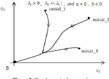
2 in the equations (3) and (4), and then repeat the step 3.For better understanding the above synergetic equations (1) and (2) (note that the equations (3) and (4) are similar) and also for answering the second question, we draw the sketch map of such equations.
Figure 1. Sketch map in the first case Figure 2. Sketch map in the second case
When satisfying that
q
1 is the order variable andq
2 is the control variable, namely
20
and
2|
1|
, the synergetic effect betweenq
1 andq
2 can be very different according to different parameter values. As Figure 1 shows, the three different initial points converge into the same point A (its coordinate(
(
1 2) / (
a b
),
1/ )
a
) with the time going by. However, differences also exist among the three paths owing to different initial points.q
2 beginning at the initial 3 point decreases at first and then goes up to the convergence point, whereas, in the other two paths,q
1 andq
2 are both increasing at the same time. While, because the parameters take different values, Figure 2 shows the contrast trend compared to Figure 1. All three paths in Figure 2 converge to the zero point (denoted by O in the Figure), although the trends of them seem to be a little different similar to the situation shown in Figure 1. From the above analysis and the two sketch maps shown in Figure 1 and Figure 2, two properties can be summarized about the synergetic effect betweenq
1 andq
2 with different parameter values.[Property 1] Given that
q
1 is the order variable and2
q
is the control variable, if
10
,a
0
andb
0
, then point( ,
q q
1 2)
will converge to(
(
1 2) / (
a b
),
1/ )
a
with time going by, although their paths can show different trends at the beginning according to the different initial points.
[Property 2] Given that
q
2 is the order variable and1
q
is the control variable, if
10
,a
0
andb
0
, then the point( ,
q q
1 2)
will converge to(0, 0)
with time going by, although their paths can show different trends at the beginning according to the different initial points.We need to explain that the two convergence points
1 2 1
(
(
) / (
a b
),
/ )
a
and(0, 0)
can be calculated out from the following steady state equations (7) and (8) induced from the equations (1) and (2), respectively.1 1
q aq q
1 20
(7)2
2
q
2bq
10
(8)It is noted that the cases of different parameter values are not confined to the above two kinds, for example,
1
0
,a
0
andb
0
, but the other cases are not very useful in our analysis, especially considering the actual data prepared for the forthcoming empirical analysis. This will be showed further in the part of empirical analysis.After the equations (3) and (4) have been calibrated based on the estimation of simultaneous equations, we can obtain the estimation values of the four parameters and judge which situation (or called which figure) the synergetic effect between
q
1 andq
2 belongs to. From the sketch map shown in the corresponding figure, we can get the answer to the second question how the two variables affect each other, namely the synergetic effect.Data preparation
Technology progress and industry convergence need to be measured firstly. They are the necessary data for further analysis and also reflect the development levels of technology progress and industry convergence in recent years. In the Introduction of this paper, we have explained why we select China’s data for this problem. In this section, we will show the details of how to measure these two variables. In all, it is an elaborated process needing more painstaking work.
Technology progress is measured by using DEA-based Malmquist index method, whose result is called TPL. Such method was proposed by Fare et al., (1994) and was found based on the DEA approach (see also Sufian et al, 2010; Wu
et al, 2013). The Malmquist index is defined on the basis of distance functions presented by Caves et al., (1982), and it measures the change of the total factor productivity (TFP) between two data points by calculating the ratio of their distances relative to a common technology. The total is decomposed into two parts: technical efficiency level and technological change. Here, what we concern is a technical efficiency level other than technological change. Accordingly, the original Malmquist index method is revised for our purpose and the DEA-based Malmquist index can be obtained by utilizing the following formula:
0.5 1 1
1 0
0
( , )
( , )
t t t
t
t t t
t
TFP D y
TFP D y
x x
where,
S
t
{( ,
x
ty
t) :
x
tcan produce }
y
t0( , ) inf{ : ( , ) }
t
t t t t y t
D y S
x x
1 1 1
0( , ) inf{ : }
t
t t t t
D y S
x
x
Specifically, the input
x
consists of labor and capital, the two factors, where labor is reflected by the number of employees and capital is reflected by the net fixed assets investment in the above model, and also the outputy
isexpressed by the operating income. The software DEAP 2.1 is a suitable tool for solving the above problem.
Considering the availability, the completeness and the reliability of the data, we select the listed companies of China as the analysis sample. So far, there are 146 ICT listed companies in China’s two main stock markets. Table 1 shows their codes and Table 2 shows their amounts in different years.
> 6 pt
Table 1
Stock codes of 146 listed ICT companies in China’s two main stock markets> 6 pt
Stock codes
000021 000938 600355 600845 600476 002153 002281 002401 300038 300085
000035 000948 600498 600850 600570 002161 002296 002405 300042 002446
000063 000977 600536 600855 600990 002184 002308 002410 300044 002465
000066 000997 600588 600050 002052 002194 002312 002416 300045 002467
000070 600037 600601 600271 002063 002195 002313 002417 300047 300096
000503 600076 600621 600392 002065 002214 002315 002421 300050 300098
000547 600105 600640 600485 002089 002230 002316 002439 300051 300101
000555 600118 600687 600487 002090 002231 002331 002449 300052 300102
000561 600122 600718 600522 002093 002232 002339 300002 300059 300104
000586 600130 600728 600571 002095 002236 002362 300010 300065 300113
000701 600171 600756 002017 002104 002253 002368 300017 300074 300162
000748 600198 600764 002027 002106 002261 002373 300025 300075
000823 600288 600770 600403 002115 002268 002376 300028 300076
000851 600289 600775 600410 002148 002279 002383 300033 300079
000892 600345 600776 600446 002151 002280 002396 300036 300081
Source: selected by the authors based on the listed company information (website:http://www.cninfo.com.cn/)
Table 2
> 6 pt
China’s listed ICT companies’ amounts during 2002–2012
>Year 2002 2003 2004 2005 2006 2007 2008 2009 2010 2011 2012
Numbers of Listed ICT
Companies 48 55 63 63 64 73 86 88 136 146 146
Source: selected by the authors based on the listed company information (website:http://www.cninfo.com.cn/)
> 6 pt
All the data (mainly
( ,
x
ty
t)
of each year) are collected from 146 listed ICT companies’ semi-annual reports from 2002 to 2012. Two things have been paid much attention to in our calculation process. The first one is that the data in the first half year of 2002 are taken as the benchmark, and all the years’ TPLs are further calculated based on this year. The purpose of doing this is to make all the TPLs to have the same benchmark so that they are comparable at different years. The approach of calculating is shown in formula (10), where n0.5, 1, 1.5, 2, . And, the second one isthat not every listed company exists at the beginning of the survey period, namely some of them went public later than some others. Thus, we make the data start year as the measurement-based year, calculate every listed ICT company’s TPL in their public duration, and then get the average of all the ICT companies’ TPLs existing in the corresponding semi-year to be the result. All the results are listed in Table 3. As the Table illustrates, China’s listed ICT industry undergoes obviously improving technology progress from 2002 to 2012.
> 6 p 2002 2002 0.5 2002 1 2002
2002
2002 2002 2002 0.5 2002 0.5
TPL n n n
n
TFP TFP TFP TFP
TFP TFP TFP TFP
(10)
Table 3
> 6 pt
China’s listed ICT industry TPL from 2002 to 2012
> 6 pt
Year 2002
fh
2002 sh
2003 fh
2003 sh
2004 fh
2004 sh
2005 fh
2005 sh
2006 fh
2006 sh
2007 fh
TPL 1,000 1,097 1,163 1,161 1,226 1,248 1,253 1,273 1,266 1,268 1,274
Year 2007
sh
2008 fh
2008 sh
2009 fh
2009 sh
2010 fh
2010 sh
2011 fh
2011 sh
2012 fh
2012 sh
TPL 1,301 1,269 1,303 1,324 1,369 1,378 1,391 1,401 1,435 1,456 1,523
Source: calculated by the authors based on the companies’ semi-year reports. Notes: fh denotes the first half year; sh denotes the second half year
We next present how to measure the industry convergence. Generally speaking, there are two streams of the literature on measuring industry convergence. One stream measures industry diversification (Teece et al, 1994; Gambardella & Torrisi, 1988), and the other measures technology relatedness (Fai & Tunzelmann, 2001). Our paper follows the latter stream, which uses patent data to analyze convergence. The technology relatedness is always taken as a significant measure for industry technology convergence (Karvonen et al, 2012), and furthermore the patent licensing data are suitable for illustrating
inter-industry technology convergence (Geum et al., 2012), which is proper for our problem.
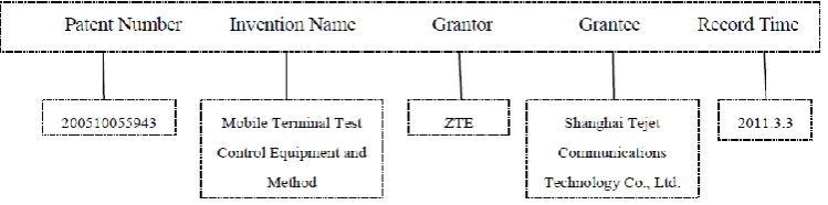
From China’s state intellectual property office (SIPO), we have got the material called patent licensing contract
records information table which records the basic information of one patent including Patent Number, Invention Name, Grantor, Grantee and Record Time. One example has been given in Figure 3. We selected data of the listed ICT companies, which have been mentioned above, from the information table, and the whole data period is from 2002 to 2012.
Figure 3. One example of the patent record in the patent licensing contract records information table
All the listed ICT companies can be divided into seven sectors: the communication equipment manufacturing sector (CEM), the computer manufacturing sector (CM), the electronic components manufacturing sector (ECM), the household and video equipment manufacturing sector (HEM), the other electronic equipment manufacturing
sector (OM), the information transmission service sector (IS), and the computer service and software sector (CS). The technology relatedness can be measured by using one transfer matrix as shown in Table 4. Here, we take the data in 2012fh (the first half year) as an example. It is noted that we make half a year as an investigation unit.
> 6 pt
Table 4
> 6 pt
ICT industry technology transfer matrix of China in 2012fh
> 6 pt
ICT sectors CEM CM ECM HEM OM IS CS
CEM 7 2 1 1 1 1 2
CM 2 1 2 0 1 0 1
ECM 1 2 13 2 0 2 0
HEM 0 1 2 15 3 0 2
OM 1 0 1 3 4 3 1
IS 0 1 0 0 0 2 0
CS 1 0 1 2 2 1 7
Source: elaborated by the authors based on the patent licensing contract records information table of China in 2012
> 6 pt
The table has 7 rows and 7 columns. Each row represents one sector’s patent penetrating into the other ICT sub-sectors, and each column illustrates patents absorbed from the responding ICT sub-sectors. The data on the diagonal line of matrix reflect technology flow within the same sector, and the data not on the diagonal line express technology convergence between different sectors. From the Table 4, we can find that 7 patents flowed within CEM sector in 2012, while 2 patents from CEM sector are absorbed by CM sector. Based on the above matrix, industry
technology convergence ratio can be calculated by the following formula:
7
7 71 1 1
TCR
nj
ia
ijn
a
njj
i ja
ijn, (11) where,a
ijn donates the number of the row i and column j in the matrix of year n, and the parameter j takes values from 1 to 7, which reflects seven sectors from CEM to CS in sequence. Then, the whole year’sTCR
n is the sum of all the individual sectors’TCR
nj. As a result, we obtain theTCR
n year by year as Table 5 shows.> 6 pt
Table 5 China’s ICT industry technology convergence ratio (TCR) from 2002 to 2012
> 6 pt
Year 2002
fh
2002 sh
2003 fh
2003 sh
2004 fh
2004 sh
2005 fh
2005 sh
2006 fh
2006 sh
2007 fh
TCR 0.1091 0.1386 0.1667 0.1759 0.2190 0.2330 0.2098 0.2583 0.2798 0.2857 0.2902 Year 2007
sh
2008 fh
2008 sh
2009 fh
2009 sh
2010 fh
2010 sh
2011 fh
2011 sh
2012 fh
2012 sh
> 6 pt
Empirical Results
Based on Data Preparation, the empirical analysis can be carried out to answer the two questions proposed in the Introduction. Before estimation methods of simultaneous
equations are selected and discussed, the two-dimensional diagram consisting of China’s ICT industry technology convergence rate and technology progress level is drawn to show the visual trend during the period from 2002 to 2012.
Figure 4. Two-dimensional diagram of TCR and TPL
In Figure 4, TCR is horizontal axis and TPL is the vertical axis, and the directions of arrows express the evolutions of the two series of variables with the years going by. On the whole, the two variables show a basically increasing trend, although some fluctuations exist. However, further technique tool is necessary to answer the two questions, since the above graph can not tell which variable the order one is and which the control one is.
As the equations (5) and (6) show, the method for estimation of the simultaneous equations is needed. Usually, three approaches are used to the system estimation of simultaneous equations, and they are three-stage least squares (3SLS) (Zellner et al., 1962), full information maximum likelihood (FIML) (Enders, 2001), and generalized method of moments (GMM) (Stock et al., 2002; Newey et al., 2009), respectively. We need to choose the most proper one of them to estimate the equations (5) and (6). It is obvious that the data are the kind of time series data, thus GMM method is the most suitable one because GMM allows random error items of simultaneous equations to have heteroscedasticity and serial correlation,
while the other two methods do not allow this. Besides, GMM has the lower restriction about the distribution of the random errors compared to the other two methods and it is also a robust estimation method. Thus, facing the features of the data selected in our study, we regard the GMM as a good method to estimate the equations.
Following the steps, null hypothesis should be given first. Firstly, we assume TCR is the order variable and TPL is the control variable, namely TCR is taken as
q t
1( )
and TPL asq t
2( )
in the equations (5) and (6). Then, it is needed to examine whether
20
and
2|
1|
according to Definition 1 given in this paper. Here, in the process of estimation,
q t
1(
1)
,q t
2(
1)
(t
2,3,
) and the constant term are considered as the tool variables, whereasq t
1( )
andq t
2( )
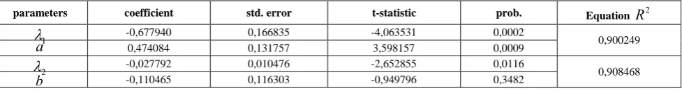
are considered as the endogenous variables. Because the number of tool variables is larger than the parameters, the whole system of equations is identifiable. Table 6 gives the results of the above assumption via Eviews 5.1 (using the GMM-time series (HAC) function) as below.> 6 pt
Table 6
Estimation results (TCR assumed to be order variable, TPL to be control variable)
6 pt
parameters coefficient std. error t-statistic prob. Equation
R
21
-0,677940 0,166835 -4,063531 0,00020,900249
a
0,474084 0,131757 3,598157 0,00092
-0,027792 0,010476 -2,652855 0,01160,908468
b
-0,110465 0,116303 -0,949796 0,3482> 6 pt
From Table 6, the coefficients of
1 and
2 do not satisfy the conditions that
2
0
and
2|
1|
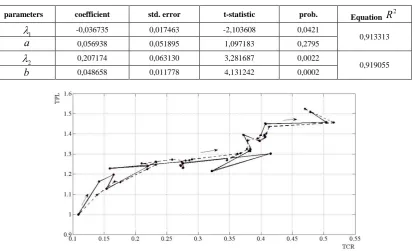
. Thus, the null hypothesis is rejected, that is to say, the estimation results can not support that TCR is the order variable and TPL is the control variable. However, the above result can not prove that its converse is right, because, in the system consisting of equations (5) and (6), it is likely that no variable is the order variable. Thus, we need to furtherTable 7 Estimation results (TPL assumed to be order variable, TCR to be control variable)
parameters coefficient std. error t-statistic prob. Equation
R
21
-0,036735 0,017463 -2,103608 0,04210,913313
a
0,056938 0,051895 1,097183 0,27952
0,207174 0,063130 3,281687 0,00220,919055
b
0,048658 0,011778 4,131242 0,0002> 6 pt
> 6 pt
Figure 5. Real numbers and fitted numbers of the two variables
> 6 pt
At this time,
20
and
2|
1|
hold as shown in Table 7, which means TPL can be seen as the order variable and TCR as the control variable according to the estimation results. Besides, judged from the values of the t-statistic and the prob. index, the coefficients of three parameters
1,
2 andb
are significant at the confidence level of 0,05. Also, the two equations both have a highR
2 which are more than 0,90. Figure 5 shows the fitted numbers and the real numbers, from which we can find the two lines are close to each other. In the whole, the estimation results are satisfied.Based on the estimation results, the equations (5) and (6) can be calibrated as>
2
TPL( 1) 1.036735 TPL( ) 0.056938 TPL( ) TCR( )
TCR( 1) 0.792826 TCR( ) 0.048658 TPL( )
t t t t
t t t
> 6 pt
Where, the underlined coefficient is not significant in the statistical sense. To sum up the results and the above simultaneous equation, two answers can be given in allusion to the two questions of this paper:
1) TPL is the order variable and TCR is the control variable; accordingly, the whole system is mainly affected by TPL. In other words, the development of technical progress (reflected by TPL) is the core factor for causing the evolution of the whole system.
2) TCR is dominated by TPL according to the second equation, whereas TCR does not affect TPL significantly since the underlined coefficient in the first equation is not significant. The relationship between the two variables indicate their synergetic effects, namely the industry technical convergence (reflected by TCR) is the outcome of the technical progress (reflected by TPL), but the
industry technical convergence on itself does not take obvious effect on the technical progress during the period we have used for empirical analysis.
Conclusions
The main objective of this study was to answer the two questions: (1) comparing industry convergence with technology progress, which one plays a dominating role in industry evolution, and (2) how industry convergence and technology progress synergistically affect industry evolution. The first contribution of this paper lies in the fact that our study is the first research to link technology progress and industry convergence in analyzing industry evolution. In contrast, previous studies (Solow, 1956; Tushman, & Anderson, 1986; Gambardella & Torrisi, 1988; Pennings & Puranam, 2001; Karvonen et al., 2010) depicted industry evolution just in one perspective, namely either technology progress or industry convergence but seldom combine them together (Bonnet & Yip, 2009). In this explorative study, we have examined industry evolution mechanism based on both industry convergence and technology progress.
However, the collected patent licensing data are more robust in illustrating industry convergence compared to the commonly used patent co-classification method (Kim & Kim, 2012). Simultaneously, we gathered 146 ICT listed company’s data to measure technology progress level. Finally, simultaneous equation estimation method (GMM time series method) is applied to empirically analyze the synergetic industry evolution process based on the established model and measured data. The conclusions and policy implications are as follows.
From 2002 to 2012, China’s ICT industry enjoys increasing convergence rate and improving technology progress level. As for the whole industry system, technology progress and industry convergence are the two endogenous factors affecting the system evolution. Our result indicates that the development of technology progress is the core factor for causing evolution of industry system, and industry convergence is the outcome of technology progress. In other words, industry synergetic evolution mechanism can be summarized that (1) technology progress is the order parameter which dominates the evolution of the system, and (2) industry convergence is the control parameter which is reflected by technology progress. These results are
somewhat in line with previous work (Bakhshi & Larsen, 2005), which has pointed that technology progress is the drive force of industry and economic growth. However, our work goes much deeper, because we have considered the new convergence trend in economic system and investigated which factor is the dominate role in the whole system by introducing the technique of synergy analysis. Note that research on industry convergence (Hacklin, 2010; Stieglitz, 2003) mainly stayed in the qualitative level previously, and few study used quantitative method to explore its role in industry growth (Curran, 2011; Karvonen et al., 2012).
The policy implication of our result is important for companies and government. It is important that the dominated role of technology progress will be sustained, even though in the environment of convergence, companies also need to focus on self-innovation, rather than only adapt to the new industry evolution trend.
Although the results are achieved from China’s ICT industry data, they may have implications for other countries. Limited by data availability, this paper only investigated the listed ICT industries from 2002 to 2012. Exploratory work on other industries and international comparisons would be directions for future research.
This paper is supported by two funds: National Social Science Funds of China(11AZD081)and National Natural Science Funds of China(71203172).
References
Bakhshi, H., & Larsen, J. (2005). ICT-specific Technological Progress in the United Kingdom. Journal of
Macroeconomics, 27(4), 648–669. http://dx.doi.org/10.1016/j.jmacro.2004.03.004.
Bonnet, D., & Yip, G. (2009). Strategy Convergence. Business Strategy Review, 20(2), 50–55. http://dx.doi.org/10.1111/j. 1467-8616.2009.00599.x.
Broring, S. (2005). The Front End of Innovation in Converging Industries: The Case of Nutraceuticals and Functional Foods. Wiesbaden,Germany: DUV. http://dx.doi.org/10.1007/978-3-322-82102-7
Caves, D.W., Christensen, L.R., & Diewert, W. E. (1982). The Economic Theory of Index Numbers and the Measurement of Input, Output and Productivity. Econometrica, 50(6), 1393–1414. http://dx.doi.org/10.2307/1913388
Curran, C. S., Broring, S., & Leker, J. (2010). Anticipating Converging Industries Using Publicly Available Data. Technological Forecasting & Social Change, 77(3), 385–395. http://dx.doi.org/10.1016/j.techfore.2009.10.002
Curran, C. S., & Leker, J. (2011). Patent Indicators for Monitoring Convergence - Examples from NFF and ICT. Technological
Forecasting & Social Change,78(2), 256–273. http://dx.doi.org/10.1016/j.techfore.2010.06.021
Dosi, G. (1982). Technological Paradigms and Technological Trajectories: A Suggested Interpretation of the Determinants and Directions of Technology Change. Research Policy, 11(3), 147–163. http://dx.doi.org/10.1016/0048-7333(82)90016-6
Dowling, M., Lechner, C., & Thielman, B. (1998). Convergence: Innovation and Change of Market Structures between Television and Online services. Electronic Markets, 8(4), 31–35. http://dx.doi.org/10.1080/10196789800000053 Duysters, G., & Hagedoorn, J. (1998).Technological Convergence in the IT Industry: The Role of Strategic Technology
Alliances and Technological Competencies. International Journal of Economics and Business, 5(3), 355–368. http://dx.doi.org/10.1080/13571519884431
Enders, C. K. (2001). The Performance of the Full Information Maximum Likelihood Estimator in Multiple Regression Models with Missing Data. Educational and Psychological Measurement, 61(5), 713–740. http://dx.doi.org/ 10.1177/0013164401615001
Fai, F. M., & Tunzelmann, N. V. (2001). Industry-Specific Competencies and Converging Technological Systems: Evidence from Patents. Structural Change and Economic Dynamics, 12(2), 141–170. http://dx.doi.org/10.1016/S0954-349X(00)00035-7
Gambardella, A., & Torrisi, S. (1998). Does Technological Convergence Imply Convergence in Markets? Evidence from the Electronics Industry. Research Policy, 27(5), 445–463. http://dx.doi.org/10.1016/S0048-7333(98)00062-6
Geum, Y., Kim, C., Lee, S. & Kim, M. (2012).Technological Convergence of IT and BT: Evidence from Patent Analysis. ETRI
Journal, 34(3), 439 –449.http://dx.doi.org/10.4218/etrij.12.1711.0010
Grossman, G. M., & Helpman, E. (1991). Quality Ladders in the Theory of Growth. Review of Economic Studies, 58(1), 43–61. http://dx.doi.org/10.2307/2298044
Haken, H. (1998). Information and Self-Organization: A Macroscopic Approach to Complex System. Berlin & New York
:Springer-verlag, 1988, 134–167. http://dx.doi.org/10.1007/978-3-662-07893-8
Hacklin, F., Marxt, C., & Fahrni, F. (2010). An Evolutionary Perspective on Convergence: Inducing a Stage Model of Inter -industryInnovation. International Journal of Technology Management, 49, 220–249. http://dx.doi.org/10.1504/IJT M.2010.029419
Karvonen, M., Lehtowaara, M., & Kassi, T. (2012). Build-up of Understanding of Technological Convergence: Evidence from Printed Intelligence Industry. International Journal of Innovation and Technology Management, 9(3) ,1094–1107. http://dx.doi.org/10. 1142/S0219877012500204
Karvonen, M., & Kassi, T. (2010). Analysis of Convergence in Paper and Printing Industry. Journal of Engineering
Management and Economics, 1(4), 269–293. http://dx.doi.org/10.1504/IJEME.2010.038647
Kim, M. S., & Kim, C. (2012). On a Patent Analysis Method for Technological Convergence. Procedia social and Behavioral
sciences, 40, 657–663. http://dx.doi.org/10.1016/j.sbspro.2012.03.245
Lei, D. T. (2000). Industry Evolution and Competence Development:The Imperatives of Technological Convergence.
International Journal of Technology Management, 19(78), 699–738. http://dx.doi.org/10.1504/IJTM.2000.002848 Lucas, R. (1988). On the Mechanics of Economic Development. Journal of Monetary Economics, 22, 342. http://dx.doi.org/10.
1016/0304-3932(88)90168-7
Newey, W. K., & Windmeijer, F. (2009). GMM with Many Weak Moment Conditions. Econometrica, 77, 687–719. http://dx.doi.org/10.3982/ECTA6224
Pennings, J. M., & Puranam, P. (2001). Market Convergence and Firm Strategy: New Directions for Theory and Research. In paper presented at the ECIS conference, Eindhoven, Netherlands.
Rosenberg, N. (1963).Technological Change in the Machine-Tool Industry,1840-1910. The Journal of Economic History, 23(4), 414–443.
Romer, P. M. (1986). Increasing Returns and Long-Run Growth. Journal of Political Economy, 94(5), 1002–1037. http://dx.doi.org/10.1086/261420
Stieglitz, N. (2003). Digital Dynamics and Types of Industry Convergence: the Evolution of the Handheld Computer Market. In J. F. Christensen (Ed.), The industrial dynamics of the new digital economy (pp. 179-208). Northampoton, MA: Edward Elgar Publishing.
Stock, J. H., Wright, J. H., & Yogo, M. (2002). A Survey of Weak Instruments and Weak Identification in Generalized Method of Moments. Journal of Business and Economics Statistics, 20, 518–529. http://dx.doi.org/10.1198/07350010 2288618658
Schumpeter, J. (1934).The Theory of Economic Development.Cambridge:Harvard University Press
Solow, R. M. (1956). A Contribution to the Theory of Economic Growth. Quarterly Journal of Economics, 70(1), 65–94. http://dx.doi.org/10.2307/1884513
Sufian, F., & Habibullah, M. S. (2010). Does Foreign Banks Entry Fosters Bank Efficiency? Empirical Evidence from Malaysia.
Inzinerine Ekonomika-Engineering Economics, 21(5), 464–474.
Teece, D., Rumelt, R., Dosi, G., & Winter, S. (1994). Understanding corporate coherence: Theory and evidence. Journal of
Economic Behavior and Organization, 23, 1–30. http://dx.doi.org/10.1016/0167-2681(94)90094-9
Tushman, M. L., & Anderson, P. (1986). Technological Discontinuities and Organizational Environments. Administrative
Science Quarterly, 31, 439–465. http://dx.doi.org/10.2307/2392832
Wan, X., Xuan,Y., & Lv, K. (2011). Measuring Convergence of China’s ICT Industry: An Input -output Analysis.
Telecommunications Policy, 35( 4), 301–313. http://dx.doi.org/10.1016/j.telpol.2011.02.003
Wu, C., Li, Y. L., Liu, Q., Wang, K. S. (2013). A Stochastic DEA Model Considering Undesirable Outputs with Weak Disposability. Mathematical and Computer Modelling, 58(5/6), 980–989. http://dx.doi.org/10.1016/j.mcm.2012.09.022 Zellner, A., & Theil, H. (1962). Three-Stage Least Squares: Simultaneous Estimation of Simultaneous Equations.
Yaya Li, Yongli Li, Yulin Zhao, Fang Wang
Kuris veiksnys dominuoja pramonės evoliucijoje? Sinergijos analize pagrįsta Kinijos informacinių ir komunikacinių technologijų (IKT) pramonės analizė
Santrauka
Pramonės evoliuciją sukėlė įvairios priežastys, tarp kurių technologijos pažanga pasitvirtino kaip svarbus veiksnys, skatinantis pramonės plėtrą. Tačiau, per pastaruosius du dešimtmečius buvo nustatyta, kad pramonės konvergencija taip pat yra naujas ir darantis įtaką reiškinys (Rosenberg, 1963). Du veiksniai: technologijų pažanga ir pramonės konvergencija, dažnai laikomi dviem pagrindiniais veiksniais, lemiančiais pramonės augimą pastaraisiais metais (Bonnet ir Yip, 2009).
Technologijų pažanga buvo pripažinta kaip svarbiausias, radikalių naujovių šaltinis pramonės šakose, nes tai skatina ekonominį augimą ir pramonės šakų plėtrą (Schumpeter, 1934; Grossman ir Helpman, 1991). Pramonės konvergencijos apibrėžimas siekia septintojo dešimtmečio pradžią. Pavyzdžiui, Rosenberg (1963), remdamasis savo darbu apie JAV mašinų gamybos įrankių pramonę, parodė, kad skirtingos pramonės šakos savo gamybos procesuose
vis labiau pasikliovė tuo pačiu technologinių gebėjimų rinkiniu ir jį pavadindavo technologijų konvergencija. Be to, Gambardella ir Torrisi (1998)
tvirtino, kad elektronikos sektorius patyrė aiškią konvergenciją dešimtajame dešimtmetyje, taip pat atrado elektronikos sektoriaus teigiamą konvergenciją ir patobulintą veiklą.
Nors šios teorijos pasiūlė logiškus pramonės evoliucijos paaiškinimus, tačiau mūsų požiūriu, jos neatskleidė evoliucijos vidinio mechanizmo, ypač, kai manome, kad pramonės augimas ne tik kilo dėl technologinės pažangos vienoje atskiroje pramonės šakoje, tačiau jam įtaką taip pat padarė pramonės šakų tarpusavio konvergencija. Taigi kyla klausimas: kuri iš jų, ar pramonės konvergencija, ar technologinė pažanga atlieka dominuojantį vaidmenį pramonės evoliucijoje? Ir ar tarp jų egzistuoja sinergijos efektas? Šiuo tyrimu planuoja atsakyti į šiuos du klausimus, ir tai sudaro šio tyrimo tikslą. Kitaip nei ankstesniuose tyrimuose, šis darbas turi tikslą ištirti pramonės sinergetinės evoliucijos mechanizmą, remiantis ir pramonės konvergencija, ir technologine pažanga. Norint atsakyti į šiuos klausimus, šiame darbe buvo sudarytos sinergetinių lygčių serijos, pagrįstos savarankiškos organizacijos
teorija ir Haken modeliu (Haken, 1988). Haken modelis yra gana žinomas sisteminių mokslų srityje, tačiau retai naudojamas inžinerinės ekonomikos
srityje, o ypač pramonės ekonomikos srityje. Kadangi ekonomikos sistema yra tikra sistema realiame gyvenime, mes planuojame pritaikyti Haken modelį,
kad išanalizuotume šią realaus pasaulio sistemą. Šiame darbe visa pramonė laikoma sistema, o technologinė pažanga ir pramonės konvergencija, gali būti laikomos dviem endogeniškais veiksniais, kurie kinta vykstant sistemos evoliucijai. Iš tikrųjų, saviorganizacijos teorija yra tinkamas metodas evoliucijos
sistemai pavaizduoti. Kalbant apie taikytą Haken modelį, jame yra dviejų rūšių parametrai: eilės parametras ir kontrolės parametras. Eilės parametras
naudojamas sistemos evoliucijai valdyti, o kontrolės parametrą valdo eilės parametras. Pritaikius šį modelį, mes galime atskirti, kuris kintamasis yra eilės parametras ir kuris yra kontrolės, taip pat mes galime sužinoti, kuris iš jų atlieka lemiamą vaidmenį sistemos evoliucijoje nagrinėjamu laikotarpiu. Taigi, modelis leidžia atsakyti į šiame darbe pateiktus klausimus.
Tiksliau sakant, mes pritaikėme saviorganizacijos metodą ir Haken modelį, norėdami sudaryti sinergetines evoliucijos lygtis. Pirma, mes išreiškėme
du kintamuosius, o tiksliau, eilės kintamąjį ir kontrolės kintamąjį matematinėmis formulėmis. Antra, nustatėme sinergetinių evoliucijos lygčių diskretizacijos formas. Trečia, mes perrašėme dvi diskretizuotas lygtis, pridėdami du likusius terminus ekonometrinei analizei. Tada mes apibendrinome empirinės analizės procesą pagal keturis pateikto modelio etapus.
Remiantis anksčiau paminėtu modeliu, šiame darbe toliau atliekamas empirinis tyrimas, renkant duomenis iš Kinijos informacinių ir komunikacinių technologijų (IKT) pramonės. IKT pramonė Kinijoje greitai vystėsi nuo dešimtojo dešimtmečio ir ypač greitai augo nuo 2002 iki 2012 metų. Taigi pasirinkti duomenys gali atskleisti akivaizdžiausią konvergenciją pramonės šakose ir galingą technologinę pažangą. Nuo 2002 iki 2012 metų, Kinijos IKT pramonė matė didėjantį konvergencijos tempą ir gerėjantį technologinės pažangos lygį. Viskas, kas paminėta anksčiau šioje pastraipoje, paaiškina, kodėl mes pasirinkome šiuos duomenis empirinei analizei.
Šiame darbe technologinė pažanga ir pramonės konvergencija yra du endogeniški veiksniai, kurie daro įtaką sistemos evoliucijai. Technologijos pažangą atspindi technologinės pažangos lygis (TPL), kuris yra įvertinamas pagal surinktus 146 kompanijų, įtrauktų į IKT sąrašą duomenis. TLP vertinimo metu, sąnaudų kintamuosius sudaro du veiksniai: darbo jėga ir kapitalas, kur darbo jėgą atspindi darbuotojų skaičius, o kapitalą atspindi investicijos į nekilnojamąjį turtą, o išeigą atspindi einamosios pajamos. TLP skaičiavimui naudojamas DEA metodas, o DEAP 2.1 programinė įranga yra tinkamas instrumentas DEA modelio sprendimui. Tuo pat metu, pramonės konvergencija yra įvertinama pagal technologijos konvergencijos tempą (TKT), kurį galima apskaičiuoti pagal surinktus Kinijos patentų licencijavimo duomenis. Tiksliau sakant, pagal Kinijos valstybinės intelektualinės nuosavybės tarnybos (VINT) duomenis, mes galime gauti medžiagą, vadinamą „patento licencijavimo sutarties įrašų informacine lentele“, kurioje įrašoma pagrindinė informacija apie patentą. Norint apskaičiuoti TKT gerai ir tiksliai, visos IKT sąrašo kompanijos yra suskirstomos į septynis sektorius taip. kad technologijos konvergencija gali būti įvertinta naudojant technologijos perdavimo matricą tarp skirtingų sektorių. Atkreipkite dėmesį į tai, kad patento analizės metodas šiame darbe, tam tikru mastu, atitinka ankstesnius darbus (Fai ir Tunzelmann, 2001; Curran ir kt., 2010; Geum, ir kt., 2012). Tačiau, mes renkamės patento licencijavimo duomenis, kurie yra patikimesni, lyginant su plačiai naudojamu patento bendro klasifikavimo metodu (Kim ir Kim, 2012). Galiausiai, yra taikomas sinchroninis lygties įvertinimo metodas (tiksliau, GMM laiko serijų metodas), norint empiriškai išanalizuoti sinergetinį pramonės evoliucijos procesą, pagrįstą sukurtu modeliu ir gautais duomenimis.
Mūsų rezultatai rodo, kad technologinės pažangos plėtra yra pagrindinis veiksnys, sukeliantis pramonės sistemos evoliuciją, o pramonės konvergencija yra technologinės pažangos rezultatas. Kitaip tariant, pramonės sinergetinės evoliucijos mechanizmą galima apibendrinti taip: (1) technologinė pažanga yra eilės parametras, kuris vyrauja sistemos evoliucijoje, ir (2) pramonės konvergencija yra kontrolės parametras, kurį atspindi technologinė pažanga. Mūsų rezultato politinė prasmė būtų svarbi ir naudinga kompanijoms ir valdžiai. Išvados galėtų būti tokios: kompanijos turėtų didinti sąnaudas mokslinio tyrimo ir projektavimo konstravimo darbams, tobulinti savarankiškus kūrybinius gebėjimus ir stiprinti pramonės technologinės pažangos lygį; iš kitos pusės, įmonės turėtų absorbuoti kitos pramonės šakos rezultatus ir tobulinti savo technologinius absorbcijos pajėgumus. Tuo pat metu, valdžios institucijos galėtų vykdyti politiką, kuri skatintų savarankiškas inovacijas pramonės šakose, stiprintų bendrą pramonės technologijos platformą, taip pat gerintų technologijų įsiskverbimą ir perdavimą tarp pramonės šakų. Ypač svarbu yra tai, kad dominuojantis technologinės pažangos vaidmuo turėtų būti nepertraukiamas net konvergencijos aplinkoje, tokiu būdu kompanijos sutelktų dėmesį į savarankiškas inovacijas, o ne tik taikytųsi prie naujos pramonės evoliucijos krypties be savarankiškų inovacijų. Apibendrinant galima teigti, kad pirmas, svarbus šio darbo įnašas yra tas, kad mūsų darbas yra pirmasis toks tyrimas, susiejantis technologinę pažangą su pramonės konvergencija analizuojant pramonės evoliuciją. Jis skiriasi nuo kitų, ankstesnių darbų (Solow, 1956; Gambardella ir Torrisi, 1988; Pennings ir Puranam, 2001; Karvonen ir kt, 2010), kuriuose buvo tiriama pramonės evoliucija tik iš vienos perspektyvos: technologinės pažangos, pramonės konvergencijos. Labai retai siedavo jas kartu (Bonnet ir Yip, 2009). Antras svarbus įnašas: pasiūlyti naują analizės metodą, atskleisti pramonės evoliucijos mechanizmą. Mes pritaikėme savarankiškos
organizacijos metodą ir Haken modelį, norėdami sudaryti sinergetines evoliucijos lygtis ir pasirinkome pramonės konvergenciją ir technologinę pažangą
kaip svarbiausius kintamuosius pramonės evoliucijos sistemoje. Nors šio darbo rezultatai yra gauti iš Kinijos IKT pramonės duomenų, jie gali turėti reikšmę kitoms šalims. Kadangi prieinami duomenys buvo riboti, šiame darbe buvo nagrinėti tik IKT pramonės sąrašo duomenys nuo 2002 iki 2012 metų. Kitų pramonės šakų ir tarptautinių organizacijų tiriamasis darbas sudarytų gaires būsimam tyrimui.
Raktažodžiai: pramonės evoliucija, pramonės konvergencija, technologijos pažanga, sinergijos analizė, Haken modelis, informacinių ir komunikacinių
technologijų pramonė, patentų duomenys, sinchroninis lygties įvertinimas, Kinija.