http://www.sciencepublishinggroup.com/j/ijber doi: 10.11648/j.ijber.20190804.13
ISSN: 2328-7543 (Print); ISSN: 2328-756X (Online)
The Stability of Population and GDP Growth: A
Comparative Analysis Among Different Nations in the
World
Aoulad Hosen
Department of Economics, National University, Gazipur, Bangladesh
Email address:
To cite this article:
Aoulad Hosen. The Stability of Population and GDP Growth: A Comparative Analysis Among Different Nations in the World. International Journal of Business and Economics Research. Vol. 8, No. 4, 2019, pp. 180-191. doi: 10.11648/j.ijber.20190804.13
Received: May 16, 2019; Accepted: June 18, 2019; Published: July 2, 2019
Abstract:
The relationship between population growth and economic growth appeared differently in different countries. It became a debated issue for one country group from another where each country group classified by their income level. This article draws on data of forty countries that is twenty seven years long with each income group consists of ten countries. For panel data analysis the study introduces some econometric tests such as Unit root test, Country Pedroni (2004) cointegration test, Phillips-Peron cross section test, Johansen normalized cointegrating tests and Vector error correction test. The outcome states that in low income countries both variables are in equilibrium and reveals positive relationship. By one percent rise in the growth of population, in the long run, for high income and upper middle income countries the growth rate of GDP will drop by 1.19 percent and 0.044 percent respectively. Meanwhile, significant positive results come from lower middle income and low income countries which were the growth of GDP upswing by 0.44 percent and 0.42 percent respectively by the one percent increase in the growth of population. In high income countries, growth of GDP falls due to rise of the growth of population but the growth of population needs 1.47 year to reach to the equilibrium.Keywords:
GDP Growth, Population Growth, Income Groups, Panel Data1. Introduction
The aim of this study is to comprehend the relationship between growth of population and growth of GDP by exercising the long-term historical data and a review of empirical works of different nations in the world. This study reflects two variables of forty countries and those countries are classified in four groups in respect to their level of national income. For any nation population plays a significant role in the growth of GDP. But it all depends on how many of them get transformed into human resource or into plain liability. In order to become a potential country, every nation requires a significant portion of its population to transform into human resource that in turns become a contributing part of the GDP and plays an important role in increasing the growth of the GDP. Generally speaking, each and every country tries to convert its population into human resource, mainly based on its distinct macroeconomic planning of the labor force. Each planning creates various
opportunities and scopes for citizens through education, training and research.
In microeconomics, the behavioral pattern and decision making processes, in terms of selling goods for a producer and buying goods for a consumer are so completely different that even the decision of a producer affects a consumer inversely. Economic activities can only move forward when both parties reach to an agreement regarding price and quantity of a particular good or service. And thus all of these economic activities and performances finally get translated into the creation of GDP, which is known as Circular flow
the basic characteristics of the labor force of a country the structure of its population and growth becomes a vital source of information, where variables such as the unemployment rate, labor force participation rate, working age population,
etcetera play key role and ensure contribution to the GDP. This study is going to examine the following countries. To understand such long running relationships between the stated variables:
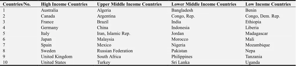
Table 1. Selected Countries in terms of Income Groups.
Countries/No. High Income Countries Upper Middle Income Countries Lower Middle Income Countries Low Income Countries
1 Australia Algeria Bangladesh Benin
2 Canada Argentina Congo, Rep. Congo, Dem. Rep.
3 France Brazil India Ethiopia
4 Germany China Indonesia Liberia
5 Italy Iran, Islamic Rep. Jordan Madagascar
6 Japan Malaysia Morocco Mali
7 Spain Mexico Nigeria Mozambique
8 Sweden Russian Federation Pakistan Nepa
9 United Kingdom South Africa Philippines Tanzania
10 United States Turkey Sri Lanka Uganda
Source: WDI, World Bank, 2018
Each group consists of ten countries and each country of the study mull over its GDP growth and population growth of 27 years raw data (from 1990 to 2017). To understand the general relationship between growth of population and growth of GDP for the respective income groups, the following frequency curves are useful:
Source: Analysis of WDI, World Bank data, 2018, in condense form
Figure 1. High Income Countries.
In the study of both variables, only China represents a steady growth of GDP against the rate of population growth but all other countries presenting uneven fluctuations over time and the gap between the variables is not high enough.
-2
0
-1
0
0
1
0
2
0
-2
0
-1
0
0
1
0
2
0
-2
0
-1
0
0
1
0
2
0
1990 2000 2010 2020 1990 2000 2010 2020
1990 2000 2010 2020 1990 2000 2010 2020
Algeria Argentina Brazil China
Iran, Islamic Rep. Malaysia Mexico Russian Federation
South Africa Turkey
Population growth (annual %)
GDP growth (annual %)
Year
Source: Analysis of WDI, World Bank data, 2018, in condense form
Figure 2. Upper Middle Income Countries.
While for upper middle income countries the study find the uneven fluctuations of both growth rates, but most of the time growth of the GDP is higher than the growth of the population.
Source: Analysis of WDI, World Bank data, 2018, in condense form
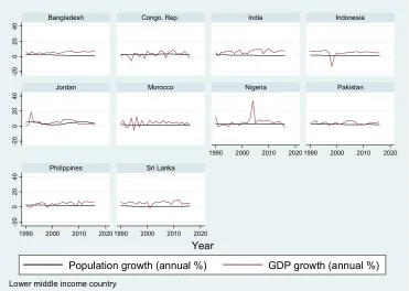
Figure 3. Lower Middle Income Countries.
-5
0
5
-5
0
5
-5
0
5
1990 2000 2010 2020 1990 2000 2010 2020
1990 2000 2010 2020 1990 2000 2010 2020
Australia Canada France Germany
Italy Japan Spain Sweden
United Kingdom United States
Population growth (annual %) GDP growth (annual %)
Year
High income country graphs by Panel id
-2
0
0
2
0
4
0
-2
0
0
2
0
4
0
-2
0
0
2
0
4
0
1990 2000 2010 2020 1990 2000 2010 2020
1990 2000 2010 2020 1990 2000 2010 2020
Bangladesh Congo, Rep. India Indonesia
Jordan Morocco Nigeria Pakistan
Philippines Sri Lanka
Population growth (annual %) GDP growth (annual %)
Year
Other than the frequency curve of Bangladesh rest nine countries that belong to the lower middle income group exhibited irregular oscillation of the growth of GDP compare to the growth rate of population. Here, the data of Bangladesh showed very optimistic and steady GDP growth trend. For that group most of the time the growth rate of GDP curves secured higher position than the growth rate of population in the comparision between two frequency lines.
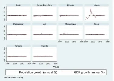
Source: Analysis of WDI, World Bank data, 2018, in condense form
Figure 4. Low Income Countries.
For the low income countries, the study showed that the fluctuation of two said variables is minimum than the other three income groups. The study observes huge fluctuations of the growth rate of GDP in the first phase of Liberia and afterwards it becomes general oscillation which is reflective of the nine other representative countries of that income group.
2. Review of Literature
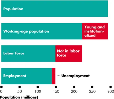
For every nation its population is the basic source of production and transforming that into human capital is a major challenge. The possibility for contributing into the GDP goes up when a country enjoys relative abundance in human capital. A segment of population, known as employed labor, directly contributes to the GDP. However, it is the rate of population growth that ensures the growth of higher volume of human capital and employed labor class irrespective of their total number. Particularly, four steps are required to ensure the transformation of population into human capital or employed labor. These are (a) Population, (b) Working-age population, (c) Labor force, and (d) Employment. Parkin (2015) [1] clearly states these steps:
The population is divided into two groups: The working-age population that is the number of people working-aged 16 years and older who are not in jail, hospital, or in other institution.
On the other hand, people who are too young to work (less than 16 years of age) or are in institutional care constitute the non-working-age population. The working-age population is again divided into two groups: (a) People in the labor force, and (b) People not in the labor force. The labor force is the sum of employed and unemployed workers. To be considered unemployed, a person must be without work and have made specific efforts to find one within the last four weeks, or waiting to be called back to a job from which he or she was laid off, or waiting to start one within the next 30 days.
The issue of labor market is extremely tricky and it has a significant impact on GDP through labor demand and labor supply (for more, please see the Appendix -2). Even, population growth itself has multidimensional effects on different related issues, such as the age structure of a country’s population, international migration, economic inequality, the size of a country’s work force, etcetera. These factors both affect and are in turn get affected by the overall economic growth.
To know the explanatory impact of population growth on the GDP rate, the human capital becomes a determining factor between the two variables. The concepts of human capital explicates by Son (2010) [2], he refers to the ability and efficiency of people to transform raw materials and capital into goods and services, and the consensus is that these skills can be learned through the educational system.
-5
0
0
5
0
1
0
0
-5
0
0
5
0
1
0
0
-5
0
0
5
0
1
0
0
1990 2000 2010 2020 1990 2000 2010 2020
1990 2000 2010 2020 1990 2000 2010 2020
Benin Congo, Dem. Rep. Ethiopia Liberia
Madagascar Mali Mozambique Nepal
Tanzania Uganda
Population growth (annual %) GDP growth (annual %)
Year
According to Jones (1996) [3] regarding the new growth theories …. such as Lucas (1988); Romer (1990); Mankiw, Romer, and Weil (1992); Barro and Sala-i-Martin (1997) ….. the accumulation of human capital through education and on-the-job training fosters economic growth by improving labor productivity, promoting technological innovation and adaptation, and by reducing fertility. Fox and Dyson (2015) [4] introduce the relationship between birth rate and per capita income. “…….(H) ousehold level consequences of high birth rates were believed to exert a significant negative effect on per capita income growth. High birth rates and rapid population growth in poor countries would divert scarce capital away from savings and investment, thereby placing a drag on economic development”. Piketty (2014) [5] observes that economic growth “…..always includes a purely demographic component and a purely economic component, and only the latter allows for an improvement in the standard of living” (p. 72). Economic growth (for more, please see the Appendix -3) is measured by percentage changes in a country’s GDP. Population growth is an important factor in the overall economic growth. Wesley and Peterson (2017) [6] find the opposite impact of population growth on GDP growth for low income countries and for high income countries:
In low-income countries, rapid population growth is likely to be unfavorable in the short and medium term because it leads to large numbers of dependent children. In the longer run, there is likely to be a demographic dividend in these countries as these young people become productive adults. It has also been argued that population growth induced by higher levels of fertility can reduce general well-being in contrast to growth resulting from declines in mortality rates. In high-income countries, population growth is low and in some cases negative, giving rise to age structures with a high proportion of elderly people in the population. The burden of supporting a large number of retired people could be eased if population growth were higher in these countries.
For low income countries GDP growth will remain domineering for at least two reasons. First, according to Piketty (2014) [5], slow economic growth may continue to be a factor in rising inequalities in the distribution of income and wealth. Second, in low-income countries it is crucial for raising the level of living and reducing global inequalities between the more prosperous industrialized countries and those that are poverty stricken, where standards of living is low and still widespread. Furthermore, the role of effort or luck of it cannot play a large role in explaining the global distribution of individual income (Milanovic, 2015) [7].
There are some conceptual schools that explore the basic relationship between population growth and GDP growth. The basic classical idea mainly based on a subsistence real wage rate, which is the minimum real wage rate needed to maintain life. Here labor supply as well as population growth determined by the minimum real wage rate. On the other hand, the neoclassical view is that the population growth rate is independent of real GDP and the real GDP growth rate.
The population growth rate equals the birth rate minus the death rate. The birth rate is determined by the opportunity cost of a woman’s time. Fall in both birth and death rate have offset each other and made the population growth rate independent of the level of income. Finally, the new growth theory holds that real GDP per person grows because of choices that people make in the pursuit of profit and that growth can persist indefinitely (Parkin, 2010) [8].
If the public and private sector initiatives regarding transforming population into human capital remain the same, that is if the cost of education, training, research, etcetra remains fixed, then population growth plays the role of explanatory variable to determine the rate of growth. Without this explanatory variable, GDP of a country gets determined by a lot of explanatory variables such as – investment in capital machineries, level of technology, alternative resource usages, external economy, and even socio-political issues might play a significant role in determining the volume of GDP. This study is based on the relationship between the growth of population and the growth of GDP growth, besides it analytically compares nations from four categories of income level.
3. Statement of the Problem
Based on both short and long run analysis this study highlights the effect of population growth on the GDP growth. To achieve the long run equilibrium this study finds out stability of two variables among the categories of four nations.
4. Objectives
1. To know the long running relationship between population growth and GDP growth among different nations.
2. To find out the countries that ensures the stability of equilibrium.
3. To find out the reasons active behind the stability.
5. Hypothesis
There exists a negative or a positive relationship between GDP growth and population growth among the four categories of nations.
6. Research Methodology
a total period of 27 years (from 1990 to 2017). This is a secondary data based study that uses data from sources like the World Development Indicators (2018) [9] and the World Bank. The selection procedure of forty countries was based on purposive sample technique and followed by the classification of the WDI and the World Bank data. Apart from those two sources the study makes good use of data gathered from authoritative research journals, periodicals, books, and online authentic sources.
To analyze the panel data and to find the results some necessary econometric tests have been incorporated here. These are Panel unit root test (without and with trend), Country Pedroni (2004) Cointegration Test, Phillips-Peron Cross Section Specific Result, Johansen Normalized Cointegrating Tests for Long-Run Coefficients Estimates and Vector Error Correction Tests for Short-Run Coefficients Estimates. The data compiled and analyzed with the support of EViews (Copyright © 1994–2009 Quantitative Micro Software, LLC) software 7.
Econometric Model
This research investigates whether there exists a long-running relationship between rate of GDP growth and the rate of population growth. In order to do this, the researcher conduct recently developed panel data unit roots for data stationary, cointegration tests and vector error correction tests. The unit root tests of panel data is an augment of the univariate time series of unit root tests. The univariate unit root tests can not easily reject the null hypothesis of panel data unit root approach. Now, Assuming the simple panel data model for GDP growth rate (gdpi t, ) with autoregressive AR (1) process.
, , 1 , ,
gdpi t =φigdpi t− +d bi i t+εi t (1)
Where, = 1, 2, 3, ……, is the cross-section dimension, = 1, 2, 3, ……, is the time dimension, εi t, is a stationary error term the bi t. term may contain vector of panel – specific means and time trend or nothing, depending on the options specified in the panel unit root test and indicates corresponding vector of coefficients of .bi t. Equation (1) can
be expressed as;
, , 1 , ,
gdpi t ρigdpi t d bi i t εi t
∆ = − + + (2)
Therefore, the null hypothesis is : =0∀ for all and the alternative hypopaper : < 0∀. In this paper, Levin, Lin, and Chu (LLC) (2002) [10] test use for common Unit root test.
6.1. The LLC Test
Since the individual unit root test has limited power against the alternative hypothesis with highly persistent deviation from equilibrium, LLC incorporates common unit root process. The null and alternative hypothesis are respectively : =0∀ and : < 0∀.
The LLC test proceeds in three main steps:
First, Augmented Dickey-Fuller (ADF) test is occupied for each cross-section by extending the model (1) and (2) with
additional lags of the dependent variable:
, , 1 , , , ,
1
i
gdp gdp d b gdp
i t i i t i i t i j i t j i t
j ρ
ρ θ ε
∆ = − + + ∑ ∆ − +
= (3)
In the second step, two auxiliary regressions are estimated: 1.
, gdpi t
∆ on
, gdp
i t j
∆ − (for = 1, …, ) and , to obtain
the residuals ˆei t, and 2.
, 1
gdp
i t− on∆gdpi t, −j and , to find out the residuals
ˆ
, 1
i t
ν − .
To control the panel-level heterogeneity across , measure
ˆ . , ˆ
ei t ei t
i
σε =
ɶ (4)
ˆ , ˆ
, 1 ˆ vi t i t
i
ν
σε =
− (5)
Where σεˆ i denotes estimated standard error from each ADF regression for = 1,., .
In the third step, the pooled OLS regression is run:
, , 1 ,
i t i t i t
εɶ =ρνɶ − +εɶ (6)
The standard -statistic for is measured as:
ˆ ˆ ( ) t se ρ ρ ρ
= (7)
In addition, the adjusted test statistic is computed as:
ˆ ˆ ( )
(0,1)
t NTS se
N T t N T µ ρ ρ ρ σ ∗ − ∗ = ⇒ ∗ ɶ ɶ ɶ (8)
Where µ∗Tɶ and σ∗Tɶ are adjustment terms of the mean and
standard deviation, Tɶ= − −T ρ 1with
1
N i
N i
ρ ρ= ∑
= , and
1 ˆ
1 N
SN Si
N i = ∑ = ɶ with ˆ ˆ ggdpi Si i σ σε = ɶ
6.2. Pedroni (2004) Test for Panel Cointegration Test
Pedroni (2004) [11] suggested seven different residual-based panel cointegration tests for testing the null hypothesis of no cointegration. The four within-dimension-based (i.e. panel- v, panel- , semi-parametric panel- t and parametric panel- t) statistics are calculated by summing up the numerator and the denominator over N cross-sections separately. The three between dimension-based (i.e. group- , semi-parametric group- and parametric- t) statistics are calculated by dividing the numerator and by summing up over N cross-sections.
The Pedeoni (2004) cointegration regression model is:
, , ,
Where, = 1, 2, 3, ……, is the cross-section dimension, = 1, 2, 3, ……, is the time dimension,pi t, is population
growth rate, εi t, is a stationary error term and the gdpi t,
dependent variable and dimensional vector of independent variables gdpi t, =gdpi t, −1+νi t, are assumed. The
cointegration vectorsβi=
(
β1, ,..., i βk i.)
the individual intercepti
α , and the trend parameter δi of cross-sections.
The null hypothesis of no cointegration for the panel cointegration test is the same for each statistic,
: 1, for all 1 ,..., N 0
H ρi = i= (10)
Whereas the alternative hypothesis for the between-dimension based and within-between-dimension based panel cointegration tests differ. The alternative hypothesis for the between-dimension-based statistics is
: 1, for all 1 ,..., N 0
H ρi < i= (11)
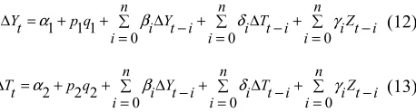
6.3. Vector Error Correction Tests
If in Johansen cointegration test detected cointreagation between the series that means there exist a long running relationship of equilibrium between explained and explanatory variables. So, researcher applies VECM for testing short running association of cointregated series. The
regression equations of VECM are as follows:
1 1 1
0 0 0
n n n
Yt p q i Yt i i Tt i i t iZ
i i i
α β δ γ
∆ = + + ∑ ∆ − + ∑ ∆ − + ∑ −
= = = (12)
2 2 2
0 0 0
n n n
Tt p q i Yt i i Tt i i t iZ
i i i
α β δ γ
∆ = + + ∑ ∆ − + ∑ ∆ − + ∑ −
= = = (13)
Where pq is the error correction component of the model that measures the speed at which prior deviations from equilibrium are corrected. VECM indicates that any short term fluctuations between explained and explanatory variables give rise to the stable long running relationship between them.
7. Results & Discussion
7.1. Unit Root Test Results: (Without Trend)
To know the long running relationship between the growth rate of GDP and the growth rate of population, the analysis incorporate panel Unit root test results, which explored and ensured the possibility of the study and analysis as well. When the persistence parameters are common across cross
-section then this type of process is called a common unit root process. Levin, Lin and Chu (LLC) (for more, please see the Appendix -4) employ this assumption. The results are
Table 2. Panel Unit root test result.
High Income Countries Upper Middle Income Countries
Lower Middle Income
Countries Low Income Countries
Variables Method Level First
difference Level First difference Level
First
difference Level
First difference GDP growth (annual %) LLC test -7.737*** -12.29*** -4.150*** -11.74*** -5.332*** -14.97*** -3.642*** -10.81*** Population growth (annual %) LLC test -1.243* -7.997*** -3.319*** -11.29*** -4.668*** -6.884*** -11.41*** -18.47***
Note: For determination of bandwidth selection by Newey-West and Bartleett kernel estimation automatically selected by Eviews software 7 (***, ** and * show level of significance at 1%, 5% and 10%, respectively).
Source: Analysis of WDI, World Bank data, 2018
From this study, three categories out of the four, namely upper middle income, lower middle income, low income (represented by thirty countries) of LLC test (without trend), showed that GDP growth (annual%) and population growth (annual%) are one percent level of significance at the first difference and the data are stationary. Even for the high income countries of LLC test delivered the evidences that GDP growth (annual%) and population growth (annual%) are significant at 1% and at 10% level and in the first difference both are significant at 1% level. So, the study uncovers that the data maintains the rule of stationary.
7.2. Panel Unit Root Test: (With Trend)
Table 3. Panel Unit Root Test Results.
High Income Countries Upper Middle Income Countries
Lower Middle Income
Countries Low Income Countries
Variables Method Level First
difference Level
First
difference Level
First
difference Level
First difference GDP growth (annual%) LLC test -7.202*** -9.750*** -3.845*** -10.26*** -5.333*** -14.97*** -2.956*** -8.794*** Population growth (annual%) LLC test -1.334* -6.486*** -9.484*** -12.37*** -4.669*** -6.885*** -16.47*** -22.63***
Note: For determination of bandwidth selection by Newey-West and Bartleett kernel estimation automatically selected by Eviews software 7 (***, ** and * show level of significance at 1%, 5% and 10%, respectively).
Near similar results found from panel unit root test with trend analysis. Here, the high income countries of LLC test provide the evidence that GDP growth (annual%) and population growth (annual%) are significant at level by 1% and by 10% respectively and in first difference both variables have unearthed high significance (1%). So, the study establishes that the data are stationary. The counties representing other three categories, namely upper middle income, lower middle income, and low income of LLC test offered the evidences that GDP growth (annual%) and population growth (annual%) both are highly significant (1%) at level and in the first difference. So, the study,
regarding two variables, established the rule of stationary for both unit root tests with trend and without trend.
7.3. Pedroni (2004) Cointegration Test
In the cointegration tests, it is considered that the null hypothesis of no cointegration must take into consideration the so-called “spurious regression” problem. Tests based on the null of cointegration must take into consideration an efficient estimation of a cointegrated relationship. To reduce exogeneity the study introduce pedroni (2004) cointegration test (for more, please see the Appendix -5)
Table 4. Country Category wisePedroni (2004) Cointegration Test Results.
High Income Countries Upper Middle Income Countries
Lower Middle Income
Countries Low Income Countries
Pedroni Test Statistics
Without Trend With Trend Without Trend With Trend Without Trend With Trend Without Trend With Trend
Statistics Statistics Statistics Statistics Statistics Statistics Statistics Statistics
within dimension within-dimension within-dimension within-dimension
Panel v-Statistic -0154576 -2.772438 -0.122204 -2.650584 -0.081423 -2.800485 -1.566530 -3.952759
Panel rho-Statistic -6.4314*** -3.5697*** -7.8894*** -6.23138*** -11.102*** -7.2450*** -10.936*** -8.6139***
Panel PP-Statistic -7.9653*** -8.5644*** -7.9330*** -9.3691*** -11.236*** -12.482*** -16.622*** -19.535***
Panel ADF-Statistic -8.3093*** -8.7296*** -7.71355*** -9.0997*** -8.4981*** -8.8290*** -14.754*** -16.918***
between-dimension between-dimension between-dimension between-dimension
Group rho-Statistic -4.9946*** -2.2938*** -5.8606*** -3.6800*** -8.3493*** -4.6181*** -7.4206*** -5.5414***
Group PP-Statistic -9.1489*** -9.3749*** -9.4636*** -10.3363*** -14.808*** -15.436*** -12.403*** -13.743***
Group ADF-Statistic -8.9295*** -8.4971*** -8.5426*** -9.1779*** -8.7195*** -8.40533*** -11.504*** -12.903***
Note: For determination of optimal lag lengths used Schwarz Information Criterion (SIC) with maximum lag length 5, bandwidth selection by Newey-West and kernel estimation by Bartlett automatically selected by Eviews software 7 (***, ** and * show level of significance at 1%, 5% and 10%, respectively). Source: Analysis of WDI, World Bank data, 2018
The results of Pedroni (2004) cointegration tests for the countries of four categories explored empirical evidence with individual intercept and individual trend test statistic within-dimension and between-dimension. The outcome of the test statistics showed that, six out of seven test statistics (Panel rho-Statistic, Panel PP-Statistic, Panel ADF-Statistic, Group rho-Statistic, Group PP-Statistic, Group ADF-Statistic) are highly significant (1% level). So, the study discovered that, there exists a long running relationship between the growth of GDP and the growth rate population.
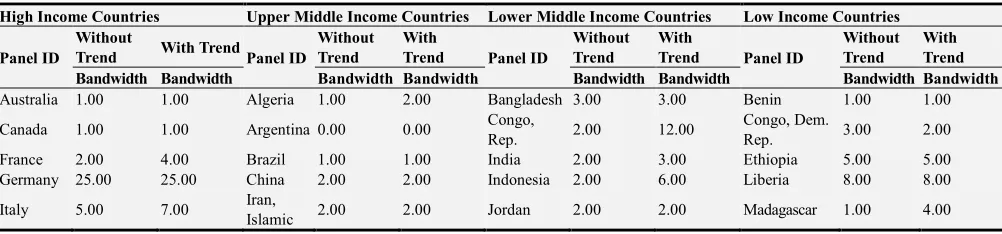
7.4. Phillips-Perron Cross Section Tests
To overcome serial correlation and heteroskedasticity, the study incorporates Phillips-Perron (PP) tests. For any serial correlation and heteroskedasticity in the errors Ut non-parametrically modifying by the Dickey Fuller (DF) test statistics through Ordinary Least Squares (OLS), but serial correlation will present a problem. To account for this, the augmented DF test’s regression includes lags of the first differences of Yt. The PP test involves fitting {∆Yt = ρYt−1+ (constant, time trend) + Ut ……(1)}, and the results are used to calculate the test statistics.
Table 5. Phillips-Perron Cross Section Specific Tests Result.
High Income Countries Upper Middle Income Countries Lower Middle Income Countries Low Income Countries
Panel ID
Without
Trend With Trend Panel ID Without Trend
With
Trend Panel ID
Without Trend
With
Trend Panel ID
Without Trend
With Trend Bandwidth Bandwidth Bandwidth Bandwidth Bandwidth Bandwidth Bandwidth Bandwidth Australia 1.00 1.00 Algeria 1.00 2.00 Bangladesh 3.00 3.00 Benin 1.00 1.00
Canada 1.00 1.00 Argentina 0.00 0.00 Congo,
Rep. 2.00 12.00
Congo, Dem.
Rep. 3.00 2.00 France 2.00 4.00 Brazil 1.00 1.00 India 2.00 3.00 Ethiopia 5.00 5.00 Germany 25.00 25.00 China 2.00 2.00 Indonesia 2.00 6.00 Liberia 8.00 8.00
Italy 5.00 7.00 Iran,
High Income Countries Upper Middle Income Countries Lower Middle Income Countries Low Income Countries
Panel ID
Without
Trend With Trend Panel ID Without Trend
With
Trend Panel ID
Without Trend
With
Trend Panel ID
Without Trend
With Trend Bandwidth Bandwidth Bandwidth Bandwidth Bandwidth Bandwidth Bandwidth Bandwidth
Rep.
Japan 5.00 5.00 Malaysia 5.00 6.00 Morocco 6.00 5.00 Mali 1.00 1.00 Spain 0.00 0.00 Mexico 6.00 6.00 Nigeria 1.00 1.00 Mozambique 0.00 0.00
Sweden 6.00 14.0 Russian
Federation 1.00 0.00 Pakistan 0.00 0.00 Nepal 9.00 7.00 United
Kingdom 4.00 4.00
South
Africa 2.00 3.00 Philippines 1.00 2.00 Tanzania 2.00 2.00 United
States 1.00 0.00 Turkey 0.00 0.00 Sri Lanka 0.00 0.00 Uganda 0.00 1.00
Source: Investigation of WDI, World Bank data, 2018
The analysis PP test found that, in the high income countries, Spain has no long running relationship between GDP and population for both with and without trend because of zero bandwidth. In the same country category, United States unearthed an indefinite picture about the said relationship by the bandwidth of zero and one for with trend and without trend respectively. For upper middle income countries the outcome of zero bandwidth showed by Argentina and Turkey, which ensured that they have no long running relationship between the growth rate of GDP and the growth rate of population. Here, the outcome of PP test showed that Russian Federation does not have any clear picture than other seven nations. Again, the said relationship cannot be established by Pakistan and Sri Lanka which belongs to the lower middle income countries. Finally, most of the countries representing as low income secured the
uttered affiliation, other than Uganda and Mozambique. Within these two countries, there was no relationship found from Mozambique and Uganda exhibited an indistinct result regarding the two variables.
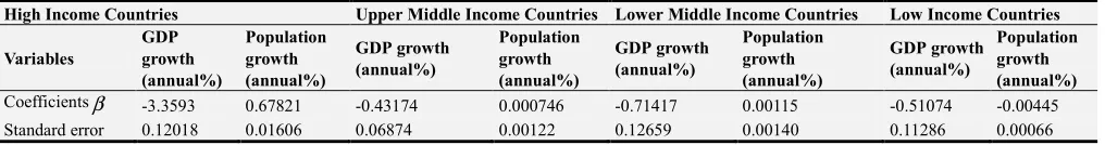
7.5. Vector Error Correction Tests
The use of Vector Error Correction Models (VECM) in the study of multivariate nonstationary time series has become a useful tools (for more, please see the Appendix -6) The main reason is that VECM allow one to describe the long-running relationships and the short-running relationships of nonstationary variables. In VECM, the cointegrating rank gives the number of independent linear stationary combinations of a multivariate nonstationary process. The autoregressive order gives the number of short-running relations.
Table 6. Vector Error Correction Tests for Short-Run Coefficients Estimates.
High Income Countries Upper Middle Income Countries Lower Middle Income Countries Low Income Countries
Variables
GDP growth (annual%)
Population growth (annual%)
GDP growth (annual%)
Population growth (annual%)
GDP growth (annual%)
Population growth (annual%)
GDP growth (annual%)
Population growth (annual%) Coefficients -3.3593 0.67821 -0.43174 0.000746 -0.71417 0.00115 -0.51074 -0.00445
Standard error 0.12018 0.01606 0.06874 0.00122 0.12659 0.00140 0.11286 0.00066
Source: Analysis of WDI, World Bank data, 2018
In the high income countries, VECM find the evidence that population growth rate showed 68 percent error in short run on the model for each year. So the model requires to correct 68% error in each year then it will reach to equilibrium in 1.47 year (=100/0.678). Meanwhile, the growth rate of GDP is already in equilibrium position (100/3.359 = 29.77, which is more than one). The study found a reverse picture about the growth rate of population regarding the upper middle income countries. In short run, growth rate of population presented 0.00075 percent error in the model for each year. By rectifying 0.00075% errors each year, it would be grasped in equilibrium in 1,33,333.33 years (=100/.00075), which is impractical and inconvenient for countries belongs to upper middle income; while, GDP growth rate of these countries are already in equilibrium (100/0.431=232, which is more than one). Again, near same remark is applicable for the category of lower middle income countries concerning the two variables. In short run, the growth rate of population
found 0.0015 percent error in the model for each year and that would not be reached to equilibrium (The analysis found an impractical result, that is it required to reach in equilibrium by 66666.67 years), while GDP growth rate already is in equilibrium position. A significant and useful result found from the countries of low income category, in the short run, result depicted that, population growth rate and GDP growth rate both are in equilibrium. It can be assessed that new portion of population of the low income countries (other than countries of Mozambique and Uganda) can directly be contributed to their GDP.
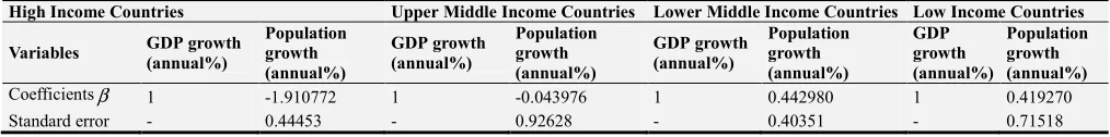
7.6. Johansen Normalized Cointegrating Tests for Long-Run Coefficients Estimates
With the development the two said variables, Johansen Normalized Cointegrating Tests can be caused permanent changes in the individual variable, there are some long-running relations of equilibrium within the individual
variables, represented by some linear combination of them. The outcomes of the Test are:
Table 7. Johansen Normalized Cointegrating Tests for Coefficients Estimates.
High Income Countries Upper Middle Income Countries Lower Middle Income Countries Low Income Countries
Variables GDP growth (annual%)
Population growth (annual%)
GDP growth (annual%)
Population growth (annual%)
GDP growth (annual%)
Population growth (annual%)
GDP growth (annual%)
Population growth (annual%) Coefficients 1 -1.910772 1 -0.043976 1 0.442980 1 0.419270 Standard error - 0.44453 - 0.92628 - 0.40351 - 0.71518
Source: Analysis of WDI, World Bank data, 2018
For high income countries, the result of Johansen normalized cointegrating test explores that, in the long run, if population growth rate rise 1 percent then the GDP growth rate will drop 1.91 percent. There is that same negative relationship assessed by upper middle income countries, where in long run if the growth rates of population increases 1 percent then the growth rate of GDP plunges down to 0.044 percentage point. Meanwhile, from the study, other two categories of countries, lower middle income and low income explored a positive relationship between the concerned variables. In lower middle income countries the result showed that, in long run, if the growth rate of population rise 1 percent then growth rate of GDP will also upswing 0.44 percent. Finally, for low income countries, the growth rate of GDP will also increase by 0.42 percent, if the growth rate of population increases by 1 percent. It can be assessed that the growth rate of population will be capitalized by augmenting the growth rate of GDP for the lower middle income countries and low income countries.
8. Findings
To know the relationship between the growth rate of population and the growth rate of GDP for forty countries of four categories, the estimates of Unit root tests results considering both with and without trend explored that the data follow the rule of stationary. The analysis discovered that, there exists a long running relationship between the growth of GDP and the growth of population growth rate by the results of Pedroni (2004) cointegration tests. The test statistics showed that, six, out of seven test statistics (Panel rho-Statistic, Panel PP-Statistic, Panel ADF-Statistic, Group rho-Statistic, Group PP-Statistic, Group ADF-Statistic) are highly significant (1% level). To overcome the problems of serial correlation and heteroskedasticity the study exercised the Phillips-Perron (PP) tests. From the examination of PP test, Spain and United States unearthed an indefinite outcome about the said relationship in the high income countries. Rest of the eight countries of that group explored a long running significant relationship between the two said variables. Again, the study did not find the aforesaid affiliation of two variables in Argentina, Turkey and Russian Federation for the upper middle income countries; Pakistan and Sri Lanka of the lower middle income countries and finally, Uganda and Mozambique of the low income countries. It can be assessed that, most of the countries, i.e. thirty one countries out of forty countries, the study findings obtained the said
relationship in the long run.
In short run, VECM find the evidence that population growth rate exhibited 68 percent error in each year for the high income countries and it requires 1.47 year to reach to the equilibrium. A significant and convenient result found from the countries of low income category, it depicted that, population growth rate and GDP growth rate both are in equilibrium. It can be judged that additional population of the low income countries (other than Mozambique and Uganda) contribute to their rate of GDP growth. In the long run, from Johansen Normalized cointegrating tests presented that by one percent rise in population growth for high income and upper middle income countries growth rate of GDP will fall by 1.19 percent and 0.044 percent respectively. Meanwhile, significant positive results found from lower middle income and low income countries which were growth of GDP upswing by 0.44 percent and 0.42 percent respectively by the one percent increase of growth of population.
9. Conclusions
The characteristics and the patterns of population appeared differently from one country group to another. Generally, it can be assessed that, the countries that belong to high income group might be successful in transforming more of their citizen into human capital than the countries that belong to comparatively low income groups. So there is a possibility for the people of high income group nations that are contributing more to their respective growth of GDP growth. From the outcome of the study, most of the countries (eight out of the ten countries) that belong to the high income group explored a long running significant relationship between the growth of GDP and the growth of population. Meanwhile, a resourceful labor force of a nation may not always be contributed to their respective growth of GDP, here, the willingness to work or willingness to leisure termed as the
backward banding supply curve (for more, please see the Appendix -7) become another issue for labor force participation of the total volume of population which belongs the countries of high income group. From the practical panel data series of different income groups of distinct country, this study mainly explored the short and long running relationships between the growth rate of population and the growth rate of GDP and its stability. After evaluating the said data through different econometric test, the policy suggestions of the research are
a)Each country can rethink about their resource allocation
regarding human capital development.
b)To ensure the stability of growth of GDP, this study has adjudicated which country with a particular population structure has been contributing more supporting role to the growth rate of GDP.
c)Find out what sorts of policy mix required among human capital, capital and rate of GDP for each countries.
Appendix
Appendix 1: Circular Flow Model
Circular flow model: “In the circular flow model, the inter-dependent entities of producer and consumer are referred to as firms and households respectively and provide each other with factors in order to facilitate the flow of income. Firms provide consumers with goods and services in exchange for consumer expenditure and "factors of production" from households” (Sloman (1999), p. 12 & Mankiw (2001) [12], p. 23.
Appendix 2: Labor Market Indicators
Figure 5. Labor Market Indicators, Source: M. Parkin (2015).
Three Labor Market Indicators: a) The unemployment rate is the percentage of the labor force that is unemployed. The unemployment rate is (Number of people unemployed/Labor force) multiplied by 100. The labor force participation rate is the percentage of the working-age population that is in the labor force. The labor force participation rate is (Labor force/Working-age population) multiplied by 100. The employment-to-population ratio is the percentage of working-age people who have jobs. The employment-to-population ratio is (Number of people employed/Working-age population) multiplied by hundred Parkin (2015) [1]. Appendix 3: Economic Growth
Economic growth is measured by changes in a country’s
Gross Domestic Product (GDP) which can be decomposed into its population and economic elements by writing it as population times per capita GDP. Expressed as percentage changes, economic growth is equal to population growth plus growth in per capita GDP. GDP is a measure of economic output and is also an indicator of national income.
Appendix 4: Unit Root Process (LLC Test)
Levin and Lin (1992) conduct an exhaustive study and develop unit root tests for the model, the model incorporates a time trend as well as individual and time-specific effects.
Appendix 5: Cointegration Test
Pedroni (1995) proposes a residual-based test for the null of cointegration for dynamic panels with multiple regressors in which the short-run dynamics and the long-run slope coefficients are permitted to be heterogeneous across individuals. The test allows for individual heterogeneous fixed effects and trend terms and no exogeneity requirements are imposed on the regressors of the cointegrating regressions [13].
Appendix 6: Multivariate Nonstationary Time Series (VECM)
In the literature, useful tools have been developed to analyze the long-running relationships, in particular the identification of the cointegrating rank. However, less attention has been given to the short-running relationships in the VECM framework, in particular the autoregressive order. Tests for the cointegrating rank depend on the autoregressive order p. Then it is important to choose the correct autoregressive order for the overall understanding of the VECM.
Appendix 7: Backward-Bending Supply Curve
“The ‘backward-bending’ supply curve is negatively sloped at high wages. That occurs because when the wage rises, individuals can both work less and earn more. They therefore choose to respond to high wages by working less. Although the labor supply curve may well slope backward in the long run, the supply curve of labor for the economy in the short run of a few years is positively sloped” (Dornbusch and Fischer, 2005) [14].
References
[1] Parkin M (2015) Microeconomics, Series: Pearson Series in Economics, Pearson, 12th Edition, London, England.
[2] Hyun H Son (2010) Human Capital Development, ADB Economics Working Paper Series No. 225, Asian Development Bank, Mandaluyong City, Manila, Philippines, www.adb.org/economics.
[4] Fox S, Dyson T (2015) Research themes: Inclusive Growth, International Growth Centre, The Ideas of Growth. University of Bristol, Economics and London School of Political Science (LSE). https://www.theigc.org/blog/is-population-growth-good-or-bad-for-economic-development/
[5] Piketty T (2014) Capital in the twenty-first century, Cambridge, MA: Belknap Press of Harvard University Press, pp. 72.
[6] Wesley E, Peterson F (2017) The Role of Population in Economic Growth, SAGE, October-December 2017: 1-15, Research Article. https://doi.org/10.1177/2158244017736094 [7] Milanovic B (2015) Global inequality of opportunity: how
much of our income is determined by where we live, Review of Economics and Statistics 97 (2): 452–460. https://doi.org/10.1162/REST_a_00432
[8] Parkin M (2010) Macroeconomics, 10th ed. Pearson Education, Inc 501 Boylston Street, Boston, MA 02116, USA. [9] World Development Indicators (2018) Data Themes, people
and Economy, The World Bank.
http://datatopics.worldbank.org/world-development-indicators/(and)
http://databank.worldbank.org/data/reports.aspx?source=world -development-indicators#
[10] Levin A, Lin C F, Chu C (2002) Unit root tests in panel data: Asymptotic and finite-sample properties. Journal of Econometrics, 108: 1–25.
[11] Pedroni P (2004) Panel cointegration: asymptotic and finite sample properties of pooled time series tests, with an application to the PPP hypopaper. Econometric Theory, 20: 575–625.
[12] Mankiw G N (2001) Principles of economics. (2nd ed.), Orlando, FL 32887-6777, Philadelphia: Harcourt College Publishers, Harcourt Inc. pp. 23 & 398-407.
[13] Pedroni P (1995) Panel cointegration: asymptotic and finite sample properties of pooled time series tests, with an application to the PPP hypopaper, Working Paper Series in Economics p. 95-013, Indiana University.