Published online October 20, 2013 (http://www.sciencepublishinggroup.com/j/acm) doi: 10.11648/j.acm.20130206.11
An effective scheme for estimating a smoother parameter
in the method of regularization
Hongmei Bao
1, Kaoru Fueda
21Graduate School of Environmental Science, Okayama University, Okayama, Japan 2Graduate School of Environmental and Life Science, Okayama University, Okayama, Japan
Email address:
[email protected] (H. Bao), [email protected] (K. Fueda)
To cite this article:
Hongmei Bao, Kaoru Fueda. An Effective Scheme for Estimating a Smoother Parameter in the Method of Regularization. Applied and Computational Mathematice. Vol. 2, No. 6, 2013, pp. 118-123. doi: 10.11648/j.acm.20130206.11
Abstract:
We had proposed a scheme for the surface approximation which consists of the estimation by the regularization method and the evaluation by generalized CV with an influence function [1]. We have to decide the value of the optimal smoother parameter which can minimize the value of the evaluation function. Among the models which have suitable parameters, we have to choose the best model using information criteria such as CV or generalized CV with an influence function (GCVIF). However, the method of GCVIF is not practical, because it requires the calculation of the inverse matrix of the hat matrix and the influence function [2]. Those calculations take a large amount of time when n increases. An efficient scheme which will take a small amount of time is required. On the other hand, there are many parameters which we have to decide.Those are the coefficients of the spline functions and the total number of knots, and positions of the parameters and a smoother parameter of the penalized term. The range of the total number of knots is decided by the total number of sample points. The range of the positions of the knots is decided by the area of the surface. However, it is difficult to estimate the range of the value of the smoother parameter. Therefore, we have to estimate it quite roughly. In this paper, we propose an effective method to estimate the range of the smoother parameter and consequently obtain the parameter precisely. We can reduce the calculation time which does not contribute to the selection of the optimal model and we can determine a more accurate and smoother parameter in a small amount of time.Keywords:
Spline Interpolation, Penalized Coefficient, Smoother Parameter, Method of Regularization, Cross-Validation1. Introduction
The smoothing spline surfaces are often used to estimate a three-dimensional shape of the surface. When we use the regularization method with the penalized term, the smoothing parameter is most important. Too large of a parameter produces a surfacethat is too flat and too small of a one causes over-fitting and creates a surface without fluency. The value of the appropriate parameter varies according to the shape of the surface to be estimated. We have to search for the appropriate range of the value of the smoothing parameter. When we have decided the set of the parameter and coefficients, we will evaluate them by the information criterion. However, it will take a long time to calculatewhen we have chosen CV. For the many sets of knots and many values of parameters we have to calculate the values of CV. However most of them don't contribute to the determination of the optimal model. We introduce a scheme which usessets that are as small as possible.
Moreover, we can obtain a more accurate value of the smoother parameter.
2. Surface Approximation by B-Splines
2.1. B-Splines
A B-spline of degree n is a function composed of a linear combination of basis B-splinesBi,nof degree n[3-5].The
m-n-1 basis B-splines of degree n can be defined, for
n=0,1,...,m-2, using the Cox-de Boor recursion formula as follows:
, 0 otherwise1 if (j=0,1, ,m-2)
, ,
, ,
0,1, , ! " 2 wherem is the total number of the knots and $ $
$% . We set the approximation for the three dimensional surface:
' , ( ∑ ∑ *.201 .0/ + ,+ - ( , (1)
wherep1, p2 is the total number of basis B-splines {Mi(x)},{Nj(y)} respectively,and these functions have the
support [ ξ+ 4, ξ+ ), [ η 4, η for the x,y direction respectively.We have to satisfy theSchoenberg-Whitney condition [6] because if there is no sample point in the domain {(x,y)| ξ+ 4 6+, 7 4 ( 7 8, then we cannot determine the parameter*+ . Usually, B-splines with order four (degree three) are used in the calculation. Along the x direction, we set the knots , 9, , .and the knots at both ends were four-folded. Therefore, the total number of basis B-splines should bep-4. At every intervalof : ,
, " 5,6, , = 3there exists four basis B-splines, as below.
, ?@ ?@BA ?@? ??@B/@ A ?@ ?@B1 , (2)
,9 ? ?@BA ? ?@ ? ?@ ?@ ?@BA ?@ ?@B/ ?@ ?@B1
? ?@B/ ? ?@ ? ?@C1
?@C1 ?@B/ ?@ ?@B/ ?@ ?@B1 ? ?@B1 ? ?@C1 ? ?@C1
?@C1 ?@B1 ?@C1 ?@B/ ?@ ?@B1, (3)
,D ? ?@B/ ? ?@B/ ? ?@ ?@C1 ?@B/ ?@ ?@B/ ?@ ?@B1
? ?@B/ ? ?@B1 ? ?@C1
?@C1 ?@B/ ?@ ?@B1 ?@C1 ?@B1 ? ?@B1 ? ?@B1 ? ?@C/
?@C1 ?@B1 ?@ ?@B1 ?@C/ ?@B1 , (4)
,E ?@C/ ?@B1 ? ??@C1@B1 A?@B1 ?@ ?@B1 . (5)
We denote the total number of knots (nx, ny) where nx and nyare the total number of knots along the x and ydirections respectively.
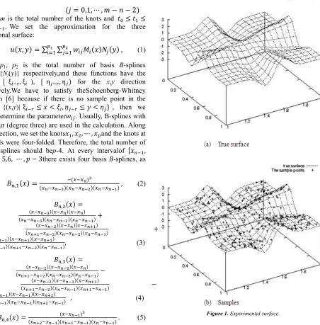
2.2. Sample Surface
To evaluate our scheme, we have made the next numerical experiment.We have used the sample surface with the equation as follows:
F 1 exp 9 (
exp 9 (exp (9 .
We have taken the randomized samples with Gaussian noise.We set the region of the samples [0,1]I[1,2] shown in Fig.1 and set n=300as the total number of samples.Using these samples, we estimated the coefficients of the models based on the various conditions.For the determination of the optimal model we evaluated the models by CV.
3. Estimation of Coefficients of B-Spline
for Regularization Method
For the nonlinear statistical modeling, the maximum penalized likelihood methods are often used [7-9].Suppose that we havenobservations J FK, K ; α 1, , "8, where FK are the response variables generated from unknown true distribution G F| having a probability density of g F| and K are the vectors of explanatory variables.We estimate w, which is a vector consisting of the unknown parameters, and determine the model F ' |* . LetQ FK| K ; R be a specified parametric model, where R is a vector of unknown parameters included in the model.The regression model with Gaussian noise is denoted as:
FK ' K|* SK , SK~- 0, U9 , V 1, , "
Q FK| K; θ 1
√2YU9expZ
JFK ' K; * 89
2U9 [ ,
where R *\U9 \.The parameter will be determined by the maximization of the penalized log-likelihood function, expressed as:
ℓ^ R ∑K0 log Q FK| K; R 9`a * (6)
As the regularized term or penalized terms H(w) with an
m-dimensional parameter vector w,various types are used depending on the dimension of explanatory variables or the purpose of the analysis.For the three-dimensional approximation we use [10]:
a * b cdd?/e/f 9
cddg/e/f 9
h i i( , (7)
and it is represented in the quadratic form:
a * *\j* (8) Therefore, (6) will be
ℓ^ R "2 log 2YU9 2U19 F * \ F * "2 `*\j* , where F F , , F \, ' K|* *\k K and B is annIm matrix composed of thebasisfunctions as:
B k \, , k \ \ .
With respect toR, differentiating ℓ^ R and setting the result equal to zero obtainsthe solution.As a result, the estimations of the parameters are:
*m \ "`Un9j \F ,
Un9 F *m \ F *m . (9)
At first, we set the constant value of o λσm9 and determine*mfor a given value of o.After we obtain the variance estimator σm9 we can then obtain the smoothing parameter λ o/σm9.
4. Evaluation of the Model
For the B-spline, the total number and the locations of the knots are important.When the knots at both ends are four-folded, the least total number of knots is ten along the x
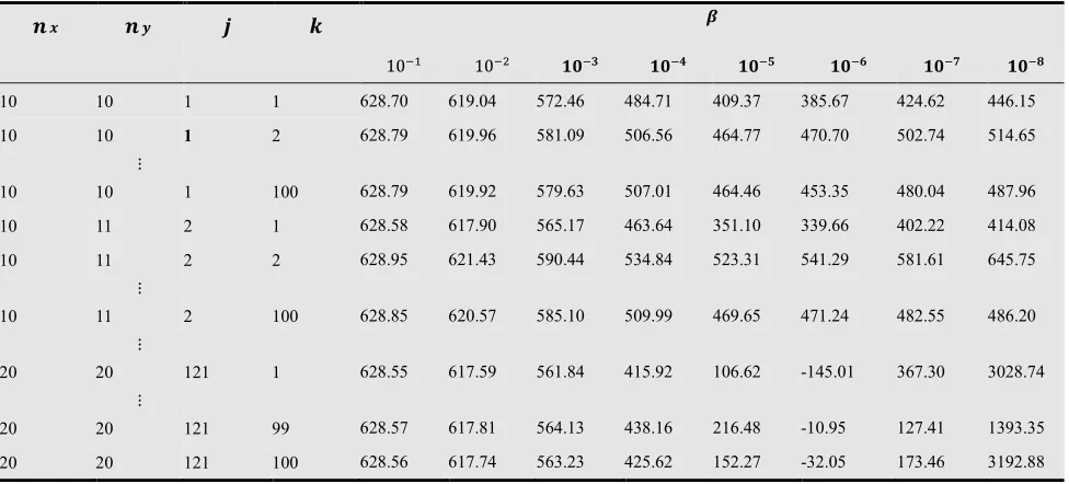
and yaxis respectively.The total number of parameters is "? 4 I "g 4 1 which consists of the coefficients of the basis and the variance, and this value should be less than the total number of the sample points, at least.We have set 300 sample points, and the adequate total number of knots along every axis is less than or equal to 20. Also, for every "?, "g), we prepared 100 sets of randomized knots generated uniformly.However, if some of them donot satisfy theSchoenberg-Whitney condition [5], then we must generate another set of knots again.Furthermore, ifsome equations of matrices made from ill-conditioned sets cannot be solved properly, then we also must generate another set of knots again.We prepared 100 solvable sets for every "?, "g) .We denote a set of knots as t,u 1,2, ,121, v 1,2, , 100 where 11 "? 10 "g 10 1 represents the number of knots and k represents the serial number of the sets which has the same total number of knots. On the other hand, we tried eight values of the smoother parameter which is the coefficient of the penalized term. We set the values of o from 10 to 10 w, so we considered 96,800 models and determined the parameters of those by the regularization method. The evaluations of the models are done by the value of CV. We use the log-likelihood for Cross-Validation (CV) as:
xy 2 z log cQ{ K, R K|f K0
∑ }log{2YUn9 K| {~• emB•|/ €m/ B• • ‚
ƒ0 . (10)
whereUn9 K, R K, 'm K are determined by the data without an V-thsample.We only tried very rough values ofo.The resultsare shown in Table 1-2.
In order to determine a better model, we need a more accurate value ofo. However, it will take much time to calculate the values of CV's, so.we studied to obtaina more efficient scheme.In these models, there are many sets of knots and o's which are not useful to determine the best model.We saved time for calculation and tried to obtain a more correct value of o and verify the validity of our scheme.
5. Optimal Smoother Parameter
5.1. Interpolation by Spline Function
For every set of knotst,u , we have only eight values of CV for o 10 , 10 9, , 10 w. Fig. 2 shows the interpolation of the value of CV by the spline function.
Let + log „… and (+ is the value of CV for +. Spline interpolation functions Q+ †+ + D
k+ + 9 ‡+ + i+, ˆ 1, 2, , - 1 are
-1 .We determine the coefficients of these functions as follows.
Q+ + Q+ + (+
Q+\ + Q+\ +
Q+\\ + Q+\\ + for ˆ 1,2, , - 2
Figure 2. Spline Interpolation.
Based on these conditions, we can obtain the coefficients by solving the next matrix equation .
Š
‹ Œ• Œ‹
Œ‹
Ž •
Œ‹
‹ Œ‹ Œ•
Ž •
•
Υ
Ž ‘
Œ’ ‹
• • Ž
‹ Œ’ ‹ Œ’ •
“ Š
”•
”‹ Ž ”’ ‹
“ Š
••
•‹
Ž
•’ ‹
“
(11)
where–+ + + , —+ 3 g…C1˜ g…
…
g… g…B1
˜…B1 .We can
determine all variables from Jk+8 as follows:
†+ k+ 3– k+ + , ‡+
(+ (+ †+–+D k+–+9
–+ .
Our aim is to obtain the value of x which gives the minimum value of the interpolated CV.If the spline
functions are only three-dimensional polynomials, we can easily differentiate them and calculate the zero points.
Q+\ 3†+ + 9 2k+ + ‡+ 0
Let ™be the zero point for every j.Instead of calculating CV's for all setst,u 1,2, ,121, v 1,2, , 100 , we select only one v v for every j, and calculate CV's for selected setst,uš 1,2, ,121 .In those sets, we make the spline interpolation and determine the minimum estimated values ! 1,2, ,121 and ™ which gives !for every set.Among them, we determine the minimum value of !and™ which gives it.We denote those values as !›2‚ and ›2‚.Then, we obtaino›2‚ 10 ?œ•ž.Using thiso›2‚,we estimate the coefficients of the estimated surface and calculate CV for all setst,u 1,2, ,121, v 1,2, , 100 .The value ofo›2‚, that is 10 ?œ•ž varies
depending on the selection ofv,and the statistical values of ›2‚ based on 100 experiments are as follows.
The result of the calculation based on the set of various values of o›2‚which include a maximum one and minimum one shows that the model tŸ ,9 is always the best.
5.2. Estimation of the Optimal
After the determination of the best set of knots, we have to determine the optimal value of smoother parameter o.We have only vaguely estimated the value of o.To obtain thebest value of CV, we calculate it based on various values of o only on the best set, which was selected above.The range of o is set from k 3U to k 3U, where bis the mean of the best ten values of ™ in Table3 andU is the standard deviation of these values.The results of these calculations are shown in Table9.
Table 1. All values of CV by previous method
¡¢ ¡£ ¤ ¥
10 10 9 •• • •• ¦ •• § •• ¨ •• © •• ª
10 10 1 1 628.70 619.04 572.46 484.71 409.37 385.67 424.62 446.15
10 10 1 2 628.79 619.96 581.09 506.56 464.77 470.70 502.74 514.65
Ž
10 10 1 100 628.79 619.92 579.63 507.01 464.46 453.35 480.04 487.96
10 11 2 1 628.58 617.90 565.17 463.64 351.10 339.66 402.22 414.08
10 11 2 2 628.95 621.43 590.44 534.84 523.31 541.29 581.61 645.75
Ž
10 11 2 100 628.85 620.57 585.10 509.99 469.65 471.24 482.55 486.20
Ž
20 20 121 1 628.55 617.59 561.84 415.92 106.62 -145.01 367.30 3028.74
Ž
20 20 121 99 628.57 617.81 564.13 438.16 216.48 -10.95 127.41 1393.35
Table2. Minimum value of CV for eacho by previous method
¡¢ ¡£ ¤ ¥ «‹ ¬ CV
13 13 37 19 10 0.003851 2.59673E+01 31.07
18 18 97 37 10 9 0.053463 1.87045E-01 40.25
20 15 66 92 10 D 0.322460 3.10116E-03 537.93
17 20 118 95 10 E 0.165861 6.02913E-04 367.40
20 15 66 92 10 - 0.048688 2.05391E-04 74.36
16 14 51 21 10 ® 0.006367 1.57050E-04 -346.11
16 14 51 21 •• © 0.002303 4.34181E-05 -441.16
19 13 43 4 10 w 0.002769 3.61129E-06 -244.25
Table3. Minimum value of CV for each j
¡¢ ¡£ ¤ ¢°±¯ ²¤
10 10 1 5.824489 384.30
10 11 2 5.585633 330.07
Ž
20 19 120 6.232998 -150.10
20 20 121 6.200994 -159.55
Table4. Statistical values of xmin
average 6.56285
median 6.55971
standard deviation 0.10246
maximum 6.85326
minimum 6.32370
Table5. Model evaluation for o%+ 10 ®.w-D9®
¡¢ ¡£ ¤ ¥ ¬ CV
16 14 71 21 0.00240204 -462.82
15 14 60 80 0.00369185 -429.77
17 14 82 79 0.00271836 -425.07
Ž
Table6. Model evaluation for o%+ 10 ®.®Ÿ9 ³
¡¢ ¡£ ¤ ¥ ¬ CV
16 14 71 21 0.00261375 -473.44
15 14 60 80 0.00391828 -457.14
16 15 72 99 0.00325389 -429.55
Ž
Table7. Model evaluation for o%+ 10 ®.-DŸ
¡¢ ¡£ ¤ ¥ ¬ CV
16 14 71 21 0.00288071 -469.07
15 14 60 80 0.00420413 -457.27
16 15 72 99 0.00356967 -441.77
Ž
Table8. Model evaluation for o%+ 10 ®.D9DŸ
¡¢ ¡£ ¤ ¥ ¬ CV
16 14 71 21 0.00364017 -439.82
16 15 72 99 0.00438565 -429.78
15 14 60 80 0.00502962 -421.37
Ž
Table9. Values of CV for randomized
´µ¶· · ¬ CV
6.66160 2.1796 I 10 Ÿ 0.00263041 -473.493
6.65547 2.2106 I 10 Ÿ 0.00264043 -473.490
6.67365 2.1200 I 10 Ÿ 0.00261131 -473.435
6.64192 2.2807 I 10 Ÿ 0.00266333 -473.407
6.64123 2.2843 I 10 Ÿ 0.00266452 -473.400
Ž
6. Conclusion
We can reduce the amount of calculations by almost one eighth. At first, we only used one set of each number of knots. Although the estimated value of o›2‚ depends on the selection of sets, we need not mind the difference because the standard deviation of ›2‚ is quite small. Based on o›2‚, we can determine the best set of knots. Also, the determination does not depend on the value of the estimatedo›2‚.
Concerning the selected optimal set of knots, we finally obtained the optimal smoother parameter o by randomization, and its effective digit became higher than the previous method.
It is our future study how to find out set a more appropriate range of o in the final step.
References
[1] Bao, H. and Fueda, K.(2013). "A New Method for the Model Selection in B-spline Surface Approximation with an Influence Function"Science Journal of Applied Mathematics and Statistics(submitted to).
[3] Cox, M.G.(1972). "The numerical evaluation of B-splines",
J. Inst. Math. Appl., 10, pp.134-149.
[4] Cox, M.G.(1975). "An algorithm for spline interpolation", J. Inst. Math. Appl.,15, pp.95-108.
[5] de Boor, C.(1972). "On calculation with B-splines", J. Approx. Theory, 6, pp.50-62.
[6] Schoenberg, I. J., Whitney, A.(1953). "On Pólya frequency functions III", Trans. Amer. Math. Soc, Vol. 74. pp. 246-259, pp. 246-259.
[7] Good, I. J. and Gaskins, R.A.(1971). "Non parametric roughness penalties for probability densities", Biometrika, Vol. 58. pp. 255-277.
[8] Good, I. J. and Gaskins, R.A.(1980). "Density estimation and bump hunting by the penalized likelihood method exemplified by scattering and meteorite data", Journal of American Standard Association, Vol. 75. pp. 42-56. [9] Green, P. J., Silverman, B. W.(1994). "Nonparametric
Regression and Generalized Linear Models", Chapman and Hall, London.