Classifier Selection using the Predicate Depth
Ran Gilad-Bachrach [email protected]
Christopher J.C. Burges [email protected]
Microsoft Research 1 Microsoft Way Redmond, WA, 98052 USA
Editor:John Shawe-Taylor
Abstract
Typically, one approaches a supervised machine learning problem by writing down an objective function and finding a hypothesis that minimizes it. This is equivalent to finding the Maximum A Posteriori (MAP) hypothesis for a Boltzmann distribution. However, MAP is not a robust statistic. We present an alternative approach by defining a median of the distribution, which we show is both more robust, and has good generalization guarantees. We present algorithms to approximate this median.
One contribution of this work is an efficient method for approximating the Tukey median. The Tukey median, which is often used for data visualization and outlier detection, is a special case of the family of medians we define: however, computing it exactly is exponentially slow in the dimension. Our algorithm approximates such medians in polynomial time while making weaker assumptions than those required by previous work.
Keywords:classification, estimation, median, Tukey depth
1. Introduction
According to the PAC-Bayesian point of view, learning can be split into three phases. First, a prior belief is introduced. Then, observations are used to transform the prior belief into a posterior belief. Finally, a hypothesis is selected. In this study, we concentrate on the last step. This allows us to propose methods that are independent of the first two phases. For example, the observations used to form the posterior belief can be supervised, unsupervised, semi-supervised, or something entirely different. The most commonly used method for selecting a hypothesis is to select the maximum a posteriori (MAP) hypothesis. For example, many learning algorithms use the following evaluation function (energy function):
E(f) =
n
∑
i=1
l(f(xi),yi) +r(f) , (1)
wherelis a convex loss function,{(xi,yi)}ni=1are the observations andris a convex regularization
term. This can be viewed as a priorPover the hypothesis class with density p(f) = Zp1e−r(f)and a posterior belief Qwith densityq(f) = 1
patho-logical examples: in Section 2.4 we give an example where the MAP classifier solution disagrees with the Bayes optimal hypothesis on every point, and where the Bayes optimal hypothesis1in fact minimizes the posterior probability. Second, the MAP framework is sensitive to perturbations in the posterior belief. That is, if we think of the MAP hypothesis as a statistic of the posterior, it has a low breakdown point (Hampel, 1971): in fact, its breakdown point is zero as demonstrated in Section 2.2.
This motivates us to study the problem of selecting the best hypothesis, given the posterior belief. The goal is to select a hypothesis that will generalize well. Two well known methods for achieving this are the Bayes optimal hypothesis, and the Gibbs hypothesis, which selects a random classifier according to the posterior belief. However the Gibbs hypothesis is non-deterministic, and in most cases the Bayes optimal hypothesis is not a member of the hypothesis class; these draw-backs are often shared by other hypothesis selection methods. This restricts the usability of these approaches. For example, in some cases, due to practical constraints, only a hypothesis from a given class can be used; ensembles can be slow and can require large memory footprint. Furthermore stochasticity in the predictive model can make the results non-reproducible, which is unacceptable in many applications, and even when acceptable, makes the application harder to debug. Therefore, in this work we limit the discussion to the following question: given a hypothesis class
F
distributed according to a posterior beliefQ, how can one select a hypothesis f ∈F
that will generalize well? We further limit the discussion to the binary classification setting.To answer this question we extend the notions of depth and the multivariate median, that are commonly used in multivariate statistics (Liu et al., 1999), to the classification setting. The depth function measures the centrality of a point in a sample or a distribution. For example, if Qis a probability measure over Rd, the Tukey depth for a point x∈Rd, also known as the half-space
depth (Tukey, 1975), is defined as
TukeyDepthQ(x|Q) = inf
Hs.t.x∈HandHis a halfspace
Q(H) . (2)
That is, the depth of a pointxis the minimal measure of a half-space that contains it.2 The Tukey depth also has a minimum entropy interpretation: each hyperplane containingxdefines a Bernoulli distribution by splitting the distribution Qin two. Choose that hyperplane whose corresponding Bernoulli distribution has minimum entropy. The Tukey depth is then the probability mass of the halfspace on the side of the hyperplane with the lowest such mass.
The depth function is thus a measure of centrality. The median is then simply defined as the deepest point. It is easy to verify that in the univariate case, the Tukey median is indeed the standard median. In this work we extend Tukey’s definition beyond half spaces and define a depth for any hypothesis class which we call the predicate depth. We show that the generalization error of a hypothesis is inversely proportional to its predicate depth. Hence, the median predicate hypothesis, orpredicate median,has the best generalization guarantee. We present algorithms for approximating the predicate depth and the predicate median. Since the Tukey depth is a special case of the predicate depth, our algorithms provide polynomial approximations to the Tukey depth and the Tukey median as well. We analyze the stability of the predicate median and also discuss the case where a convex evaluation functionE(f)(see Equation (1)) is used to form the posterior belief. We show that in
1. The Bayes optimal hypothesis is also known as the Bayes optimal classifier. It performs a weighted majority vote on each prediction according to the posterior.
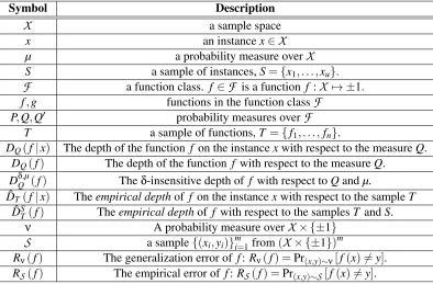
Symbol Description
X
a sample spacex an instancex∈
X
µ a probability measure over
X
S a sample of instances,S={x1, . . . ,xu}.
F
a function class. f ∈F
is a function f :X
7→ ±1. f,g functions in the function classF
P,Q,Q′ probability measures over
F
T a sample of functions,T ={f1, . . . ,fn}.DQ(f|x) The depth of the function f on the instancexwith respect to the measureQ. DQ(f) The depth of the function f with respect to the measureQ.
DδQ,µ(f) Theδ-insensitive depth of f with respect toQandµ. ˆ
DT(f|x) Theempirical depthof f on the instancexwith respect to the sampleT ˆ
DST(f) Theempirical depthof f with respect to the samplesT andS.
ν A probability measure over
X
× {±1}S
a sample{(xi,yi)}mi=1from(X
× {±1})m
Rν(f) The generalization error of f:Rν(f) =Pr(x,y)∼ν[f(x)6=y].
RS(f) The empirical error of f:RS(f) =Pr(x,y)∼S[f(x)6=y].
Table 1: A summary of the notation used in this work
this special case, the average hypothesis has a depth of at least1/e, independent of the dimension.
Hence, it enjoys good generalization bounds.
In the first part of this work we introduce the notion of predicate depth. We discuss its prop-erties and contrast them with the propprop-erties of the MAP estimator. In the second part we discuss algorithmic aspects. We address both the issues of approximating depth and of approximating the deepest hypothesis, that is, the predicate median. Table 1 contains a summery of the notation we use.
2. The Predicate Depth: Definitions and Properties
In this study, unlike Tukey who used the depth function on the instance space, we view the depth function as operating on the dual space, that is the space of classification functions. Moreover, the definition here extends beyond the linear case to any function class. The depth function measures the agreement of the function fwith the weighted majority vote onx. A deep function is a function that will always have a large agreement with its prediction among the class
F
.Definition 1 Let
F
be a function class and let Q be a probability measure overF
. The predicate depth of f on the instance x∈X
with respect to Q is defined asDQ(f|x) = Pr
g∼Q[g(x) = f(x)] .
The predicate depth of f with respect to Q is defined as
DQ(f) =inf
The Tukey-Depth is a special case of this definition as discussed in section 2.1. We can now define the predicate median:
Definition 2 Let
F
be a function class and let Q be a probability measure overF
. f∗is a predicate median ofF
with respect to Q if∀f∈
F
, DQ(f)≤DQ(f∗) .We show later, in Theorem 13, that if
F
is closed then the median always exists, for every probability measureQ. The depthDQ(f)is defined as the infimum over all pointsx∈X
. However, for our applications, we can tolerate some instancesx∈X
which have small depth, as long as most of the instances have large depth. Therefore, we define theδ-insensitive depth:Definition 3 Let
F
be a function class and let Q be a probability measure overF
. Let µ be a probability measure overX
and letδ≥0. Theδ-insensitive depth of f with respect to Q and µ is defined asDδQ,µ(f) = sup X′⊆X,µ(X′)≤δ
inf
x∈X\X′DQ(f|x) .
Theδ-insensitive depth function relaxes the infimum in the depth definition. Instead of requiring that the function f always have a large agreement in the class
F
, theδ-insensitive depth makes this requirement on all but a set of the instances with probability massδ.With these definitions in hand, we next provide generalization bounds for deep hypotheses. The first theorem shows that the error of a deep function is close to the error of the Gibbs classifier.
Theorem 4 Deep vs. Gibbs
Let Q be a measure on
F
. Letνbe a measure onX
×{±1}with the marginal µ onX
. For every f the following holds:Rν(f)≤
1 DQ(f)
Eg∼Q[Rν(g)] (3)
and
Rν(f)≤ 1
DδQ,µ(f)Eg∼Q[Rν(g)] +δ . (4)
Note that the termEg∼Q[Rν(g)]is the expected error of the Gibbs classifier (which is not
neces-sarily the same as the expected error of the Bayes optimal hypothesis). Hence, this theorem proves that the generalization error of a deep hypothesis cannot be large, provided that the expected error of the Gibbs classifier is not large.
Proof For everyx∗∈
X
we have that Prg∼Q,(x,y)∼ν[g(x)6=y|x=x
∗]
≥ Pr
g∼Q,(x,y)∼ν[f(x)6=yandg(x) =f(x)|x=x
∗]
= Pr
(x,y)∼ν[f(x)6=y|x=x
∗] Pr
g∼Q,(x,y)∼ν[g(x) =f(x)|x=x
∗and f(x)6=y]
= Pr
(x,y)∼ν[f(x)6=y|x=x
∗] Pr
g∼Q,(x,y)∼ν[g(x) =f(x)|x=x
∗]
= Pr
(x,y)∼ν[f(x)6=y|x=x
∗]D
Q(f|x∗)≥ Pr
(x,y)∼ν[f(x)6=y|x=x
First we prove (4). Define the setZ=nx :DQ(f|x) <DδQ,µ(f)
o
. Clearlyµ(Z)≤δ. By slight abuse of notation, we define the functionZ(x)such thatZ(x) =1 ifx∈Z andZ(x) =0 ifx∈/Z. With this definition we have
1
DδQ,µ(f)Eg∼Q[Rν(g)] +δ ≥ Ex ∗∼µ
"
1
DδQ,µ(f)g∼Q,(Prx,y)∼ν[g(x)6=y|x=x
∗] +Z(x∗)
#
≥ Ex∗∼µ
"
1
DδQ,µ(f)(x,Pry)∼ν[f(x)6=y|x=x
∗]D
Q(f|x∗) +Z(x∗)
#
≥ Ex∗∼µ
Pr
(x,y)∼ν[f(x)6=y|x=x
∗]
=Rν(f) .
(3) follows in the same way by setting bothZandδto be zero.
Theorem Deep vs. Gibbs (Theorem 4) bounds the ratio of the generalization error of the Gibbs classifier and the generalization error of a given classifier as a function of the depth of the given classifier. For example, consider the Bayes optimal classifier. By definition, the depth of this clas-sifier is at least one half; thus Theorem 4 recovers the well-known result that the generalization error of the Bayes optimal classifier is at most twice as large as the generalization error of the Gibbs classifier.
Next, we combine Theorem Deep vs. Gibbs (Theorem 4) with PAC-Bayesian bounds (McAllester, 1999) to bound the difference between the training error and the generalization error. We use the version of the PAC-Bayesian bounds in Theorem 3.1. of Germain et al. (2009).
Theorem 5 Generalization Bounds
Letνbe a probability measure on
X
× {±1}, let P be a fixed probability measure onF
chosen a priori, and letδ,κ>0. For a proportion1−δof samplesS
∼νm,∀Q,∀f,Rν(f)≤
1
(1−e−κ)D
Q(f)
κEg∼Q[RS(g)] + 1 m
KL(Q||P) +ln1
δ
.
Furthermore, for everyδ′>0, for a proportion1−δof samples
S
∼νm,∀Q,∀f,Rν(f)≤
1
(1−e−κ)DδQ′,µ(f)
κEg∼Q[RS(g)] + 1 m
KL(Q||P) +ln1
δ
+δ′ ,
where µ is the marginal ofνon
X
.Proof Applying the bounds in Theorem 4 to the PAC-Bayesian bounds in Theorem 3.1 of Germain et al. (2009) yields the stated results.
2.1 Depth for Linear Classifiers
In this section we discuss the special case where the hypothesis class consists of linear classifiers. Our goal is to show that deep functions exist and that the Tukey depth is a special case of the predicate depth. To that end we use a variant of linear classifiers calledlinear threshold functions. We denote byS=x∈Rd : kxk=1 the unit sphere. In this setting
F
=RdandX
=S×Rsuchthat f ∈
F
operates onx= (xv,xθ)∈X
by f(x) =sign(f·xv−xθ).3 One can think of an instancex∈
X
as a combination of a direction, denoted byxv, and an offsetxθ.Theorem 6 Let
X
=S×R andF
be the class of linear threshold functions overX
. Let Q be a probability measure overF
with density function q(f) such that q(f) = 1Zexp(−E(f))where E(f)is a convex function. Let f∗=Ef∼Q[f]. Then DQ(f∗)≥1/e.
Proof From the definition ofq(f)it follows that it is log-concave. Borell (1975) proved thatQis log-concave if and only ifqis log-concave. Hence, in the setting of the theorem,Qis log concave. The Mean Voter Theorem of Caplin and Nalebuff (1991) shows that if f is the center of gravity of Qthen for everyx,DQ(f|x)≥1/eand thus the center of gravity ofQhas a depth of at least1/e(eis Euler’s number). Note that since
F
=Rdthen the center of gravity is inF
.Recall that it is common practice in machine learning to use convex energy functions E(f). For example, SVMs (Cortes and Vapnik, 1995) and many other algorithms use energy functions of the form presented in (1) in which both the loss function and the regularization functions are convex, resulting in a convex energy function. Hence, in all these cases, the median, that is the deepest point, has a depth of at least1/e.4 This leads to the following conclusion:
Conclusion 1 In the setting of Theorem 6, let f∗=Ef∼Q[f]. Let νbe a probability measure on
X
× {±1}, let P be a probability measure ofF
and letδ,κ>0. With a probability greater than 1−δover the sampleS
sampled fromνm:Rν(f∗)≤
e
(1−e−κ)
κEg∼Q[RS(g)] + 1 m
KL(Q||P) +ln1
δ
.
Proof This results follows from Theorem 5 and Theorem 6.
We now turn to show that the Tukey depth is a special case of the predicate depth. Again, we will use the class of linear threshold functions. Since
F
=Rdin this case we will treat f ∈F
both as a function and as a point. Therefore, a probability measureQ overF
is also considered as a probability measure overRd. The following shows that for any f ∈F
, the Tukey-depth of f andthe predicate depth of f are the same.
Theorem 7 If
F
is the class of threshold functions then for every f∈F
: DQ(f) =TukeyDepthQ(f) .3. We are overloading notation here: fis treated as both a point inRdand a function f(x):S×R→ ±1.
Proof Every closed half-spaceHinRd is uniquely identified by a vectorzH∈Sorthogonal to its
hyperplane boundary and an offsetθH such that
H={g :g·zH≥θH} .
In other words, there is a 1−1 correspondence between half-spaces and points inS×Rsuch that
H7→(zH,θH)and such that
g∈H ⇔ g((zH,θH))≡sign(g·zH−θH) =1 .
The Tukey depth of f is the infimum measure of half-spaces that contain f:
TukeyDepthQ(f) = inf
H:f∈HQ(H) = x:finf(x)=1Q{g :g(x) =1} = inf
x:f(x)=1DQ(f|x) ≥ DQ(f) .
Hence, the Tukey depth cannot be larger than the predicate depth.
Next we show that the Tukey depth cannot be smaller than the predicate depth for if the Tukey depth is smaller than the predicate depth then there exists a half spaceH such that its measure is smaller than the predicate depth. Letx= (zH,θH). Since f∈Hthen f(x) =1 and thus
DQ(f)>Q(H) =Q{g :g(x) =1}=DQ(f|x)≥DQ(f)
which is a contradiction. Therefore, the Tukey depth can be neither smaller nor larger than the predicate depth and so the two must be equal.
2.2 Breakdown Point
We now turn to discuss another important property of the hypothesis selection mechanism: the breakdown point. Any solution to the hypothesis selection problem may be viewed as a statistic of the posteriorQ. An important property of any such statistic is its stability: that is, informally, by how much mustQ change in order to produce an arbitrary value of the statistic? This is usually referred to as the breakdown point (Hampel, 1971). We extend the definition given there as follows:
Definition 8 LetEstbe a function that maps probability measures to
F
. For two probability mea-sures Q and Q′ letδ(Q,Q′)be the total variation distance:δ Q,Q′=supQ(A)−Q′(A)
:A is measurable .
For every function f ∈
F
let d(Est,Q,f)be the distance to the closest Q′such thatEst(Q′) = f :d(Est,Q,f) =inf
δ Q,Q′
:Est Q′
= f .
The breakdownEstat Q is defined to be
breakdown(Est,Q) =sup f∈F
This definition may be interpreted as follows; ifs=breakdown(Est,Q)then for every f ∈
F
, we can force the estimatorEstto use f as its estimate by changingQby at mostsin terms of total variation distance. Therefore, the larger the breakdown point of an estimator, the more stable it is with respect to perturbations inQ.As mentioned before, our definition of the breakdown point for an estimator stems from the work of Hampel (1971) who was the first to introduce the concept. Since then, different modifications have been suggested to address different scenarios. Davies and Gather (2005) discuss many of these definitions. He (2005) noted that one can make the breakdown point trivial, for instance, ifEst
is a fixed estimator that is not affected by its input, it has the best possible breakdown point of 1. Moreover, it suffices to have a single function f that cannot be produced as the output of Estto make the above definition trivial. To prevent these pathologies, Definition 8 should only be used whenEstis such that for every f there existsQ′ for whichEst(Q′) = f which is the case for the estimators we study here.
The following theorem lower bounds the stability of the median estimator as a function of its depth.
Theorem 9 Let Q be a posterior over
F
. LetX′ = {x∈
X
s.t.∀f1,f2∈F
, f1(x) = f2(x)} andp = inf
x∈X\X′,y∈{±1}Q{f : f(x) =y} .
If d is the depth of the median for Q thenbreakdown(median,Q)≥d−2p.
Proof Letε>0. There exists ˆf and ˆxsuch thatQf : f(xˆ) =fˆ(xˆ) <p+ε. Let f∗be the median ofQ. LetQ′ be such that ˆf is the median ofQ′,so that
DQ′(f∗)≤DQ′ fˆ .
Note that for every f we have that
|DQ(f)−DQ′(f)| ≤δ Q,Q′ .
This follows since
|DQ(f)−DQ′(f)|=
infx Q
f′ : f′(x) =f(x) −inf x Q
′
f′ : f′(x) = f(x)
≤δ Q,Q′
.
SinceDQ fˆ
<p+εthen
d−δ Q,Q′
≤DQ′(f∗)≤DQ′ fˆ<p+ε+δ Q,Q′ .
Hence
δ Q,Q′>d−p−ε
2 and thus
breakdown(median,Q)>d−p−ε
Since this is true for everyε>0 it follows that
breakdown(median,Q)≥d−p
2 .
2.3 Geometric Properties of the Depth Function
In this section we study the geometry of the depth function. We show that the level sets of the depth functions are convex. We also show that if the function class
F
is closed then the median exists. First, we define the termconvex hullin the context of function classes:Definition 10 Let
F
be a function class and let g,f1, . . . ,fn∈F
. We say that g is in the convex-hull of f1, . . . ,fnif for every x there exists j∈1, . . . ,n such that g(x) = fj(x).Theorem 11 Convexity
Let
F
be a function class with a probability measure Q. If g is in the convex-hull of f1, . . . ,fn thenDQ(g)≥min
j DQ(fj) . Furthermore, if µ is a measure on
X
andδ≥0thenDδQ,µ(g)≥min j D
δ n,µ Q (fj) .
Proof Letgbe a function. Ifgis in the convex-hull of f1, . . . ,fnthen for everyxthere exists jsuch thatg(x) = fj(x)and hence
DQ(g|x) =DQ(fj|x)≥min
j DQ(fj) ,
thusDQ(g)≥minjDQ(fj) .Forδ>0 let
∆ = nx :DQ(g|x)≤DδQ,µ(g)
o
and for j=1, . . . ,n
∆j=
x∈∆ : fj(x) =g(x) .
Sincegis in the convex-hull of f1, . . . ,fnimplies that∪j∆j=∆and therefore
∑
j
µ(∆j)≥µ(∆)≥δ .
Hence, there exists jsuch thatµ(∆j)≥δ/nwhich implies that
DδQ,µ(g)≥D δ n,µ
Q (fj)≥minj D δ n,µ Q (fj) .
Definition 12 A function class
F
isclosedif for every sequence f1,f2, . . .∈F
there exists f∗∈F
such that for every x∈
X
, iflimn→∞fn(x)exists then f∗(x) =limn→∞fn(x).With this definition in hand we prove the following:
Theorem 13 If
F
is closed then the median ofF
exists with respect to any probability measure Q.Proof LetD=supfDQ(f)and let fn be such thatDQ(fn)>D−1/n. Let f∗∈
F
be the limit of the series f1,f2, . . .. We claim thatDQ(f∗) =D. SinceDis the supermum of the depth values, it is clear thatDQ(f∗)≤D. Note that from the construction of f∗we have that for everyx∈X
and everyN there existsn>N such that f∗(x) = fn(x). Therefore, ifDQ(f∗)<Dthen there existsx such thatDQ(f∗|x)<D. Hence, there is a subsequencenk→∞such that fnk(x) = f∗(x)and thusDQ(fnk)≤DQ(fnk|x) =DQ(f∗|x)<D.
But this is a contradiction since limk→∞DQ(fnk) =D. Hence, for everyx,DQ(f∗|x)≥Dand thus DQ(f∗)≥Dwhich completes the proof.
2.4 The Maximum A Posteriori Estimator
So far, we have introduced the predicate depth and median and we have analyzed their properties. However, the common solution to the hypothesis selection problem is to choose the maximum a posteriori estimator. In this section we point out some limitations of this approach. We will show that in some cases, the MAP method has poor generalization. We also show that it is very sensitive in the sense that the breakdown point of the MAP estimator is always zero.
2.4.1 LEARNING ANDREGULARIZATION
The most commonly used method for selecting a hypothesis is to select the maximum a posteriori (MAP) hypothesis. For example, in Support Vector Machines (Cortes and Vapnik, 1995), one can view the objective function of SVM as proportional to the log-likelihood function of an exponential probability. From this perspective, the regularization term is proportional to the log-likelihood of the prior. SVM, Lasso (Tibshirani, 1994) and other algorithms use the following evaluation function (energy function):
E(f) =
n
∑
i=1
l(f(xi),yi) +r(f) ,
wherelis a convex loss function,{(xi,yi)}ni=1are the observations andris a convex regularization
term. This can be viewed as if there is a priorPover the hypothesis class with a density function
p(f) = 1
Zp
e−r(f),
and a posterior beliefQwith a density function
q(f) = 1
Zq
e−E[f] .
2.4.2 THEMAP ESTIMATORCANGENERALIZEPOORLY
Since the MAP estimator looks only at the peak of the distribution it can be very misleading. Here we give an example for which the MAP estimator disagrees with the Bayes optimal hypothesis on every instance while the median hypothesis agrees with the Bayes optimal hypothesis everywhere. Moreover, the Bayes optimal hypothesis happens to be a member of the hypothesis class. Therefore, it is also the predicate median. Hence, in this case, the MAP estimator fails to represent the belief. The rest of this sub-section is devoted to explaining the details of this example.
Assume that the sample space
X
is a set of N discrete elements indexed by integers 1, ...,N.To simplify the exposition we will collapse notation and take
X
={1, ...,N}.The function classF
consists ofN+1 functions defined as follows: for everyi∈ {1, . . . ,N−1} the function fiis defined to befi(x) =
(
1 ifx≡iorx≡i+1
0 otherwise .
Additionally,
F
contains the constant functions f− and f+ that assign the values 0 and 1,respec-tively, to every input. Furthermore, assume that there is ε random label noise in the system for some 0<ε<1/2, and that no further information is available. Thus, the prior is the non-informative
uniform prior over theN+1 functions.
Assume that a training set consisting of just two examples is available, where the examples are(x1=1,y1=1) and(x2=3,y2 =1). Given theε random label noise, the posterior is easily
computed as
Q{f+}=
(1−ε)2
Z , Q(f−) =
ε2
Z, Q{fi=1,2,3}=
ε(1−ε)
Z ,Q{fi>3}=
ε2
Z whereZis the partition function. Note that under this posterior, for everyx,
Pr
f∼Q[f(x) =1]≤
(1−ε)2+2ε(1−ε)
Z =
1−ε2
Z
while
Pr
f∼Q[f(x) =0]≥
(N−2)ε2
Z .
Therefore, if N>1+1/ε2, for anyx, the probability that it is assigned class 0 is larger than the
probability that it is assigned class 1. Therefore the Bayes classifier is the function f−. Since the Bayes classifier is in the function class, it is also the predicate median. However, the MAP estimator is the function f+. Thus in this case the MAP estimator disagrees with the Bayes optimal hypothesis
(and the predicate median) on the entire sample space. Note also that the Bayes optimal hypothesis f0has the lowest density in the distributionQ. Hence, in this case, the minimizer of the posterior is
a better estimator than the maximizer of the posterior.
2.4.3 THEBREAKDOWNPOINT OF THEMAP ESTIMATOR
Algorithm 1 Depth Estimation Algorithm Inputs:
• A sampleS={x1, . . . ,xu}such thatxi∈
X
• A sampleT ={f1, . . . ,fn}such that fj∈
F
• A function f
Output:
• DˆST(f)- an approximation for the depth of f
Algorithm:
1. fori=1, . . . ,ucompute ˆDT(f|xi) =1n∑j1fj(xi)=f(xi) 2. return ˆDST(f) =miniDˆ(f|xi)
In order for the MAP estimator to be well defined, assume thatQis a Lebesgue measure such thatqis the density function of Qandq is bounded by some finiteM. Let f0∈
F
and considerQ′with the density function:
q′(f) =
(
M+1 if f= f0
q(f) otherwise .
While the total variation distance between QandQ′ is zero, the MAP estimator forQ′ is f0.
Therefore, for every f0 we can introduce a zero measure change toQthat will make f0the MAP
estimator. Hence, the breakdown point of the MAP estimator is zero.
3. Measuring Depth
So far, we have motivated the use of depth as a criterion for selecting a hypothesis. Finding the deep-est function, even in the case of linear functions, can be hard but some approximation techniques have been presented (see Section 4.5). In this section we focus on algorithms that measure the depth of functions. The main results are an efficient algorithm for approximating the depth uniformly over the entire function class and an algorithm for approximating the median.
We suggest a straightforward method to measure the depth of a function. The depth estimation algorithm (Algorithm 1) takes as inputs two samples. One sample,S={x1, . . . ,xu}, is a sample of points from the domain
X
. The other sample,T ={f1, . . . ,fn}, is a sample of functions fromF
. Given a function f for which we would like to compute the depth, the algorithm first estimates its depth on the pointsx1, . . . ,xu and then uses the minimal value as an estimate of the global depth. The depth on a pointxi is estimated by counting the fraction of the functions f1, . . . ,fn that make the same prediction as fon the pointxi. Since samples are used to estimate depth, we call the value returned by this algorithm, ˆDST(f), the empirical depth of f.depth. Moreover, this estimate is uniformly good over all the functions f ∈
F
. This will be an essential building block when we seek to find the median in Section 3.1.Theorem 14 Uniform convergence of depth
Let Q be a probability measure on
F
and let µ be a probability measure onX
. Letε,δ>0. For every f ∈F
let the function fδbe such that fδ(x) =1if DQ(f|x)≤DδQ,µ(f)and fδ(x) =−1 other-wise. LetF
δ={fδ}f∈F .AssumeF
δhas a finite VC dimension d<∞and defineφ(d,k) =∑di=0 ki
if d<k,φ(d,k) =2k otherwise. If S and T are chosen at random from µuand Qnrespectively such that u≥8/δthen with probability
1−uexp −2nε2
−φ(d,2u)21−δu/2 the following holds:
∀f∈
F
, DQ(f)−ε≤DQ0,µ(f)−ε≤DˆST(f)≤Dδ,µ Q (f) +ε
whereDˆST(f)is the empirical depth computed by the depth measure algorithm.
First we recall the definition ofε-nets of Haussler and Welzl (1986):
Definition 15 Let µ be a probability measure defined over a domain
X
. Let R be a collection of subsets ofX
. Anε-net is a finite subset A⊆X
such that for every r∈R, if µ(r)≥εthen A∩r6=/0.The following theorem shows that a random set of points forms anε-net with high probability if the VC dimension ofRis finite.
Theorem 16 Haussler and Welzl, 1986, Theorem 3.7 thereinLet µ be a probability measure de-fined over a domain
X
. Let R be a collection of subsets ofX
with a finite VC dimension d. Letε>0and assume u≥8/ε. A sample S={xi}u
i=1selected at random from µuis anε-net for R with a
probability of at least1−φ(d,2u)21−εu/2.
Proof of Theorem 14
By a slight abuse of notation, we use fδto denote both a function and a subset of
X
that includes every x∈X
for which DQ(f|x)≤DδQ,µ(f). From Theorem 16 it follows that with probability≥1−φ(d,2u)21−δu/2 a random sampleS={xi}ui=1is aδ-net for{fδ}f∈F. Since for every f ∈
F
we haveµ(fδ)≥δwe conclude that in these cases,∀f∈
F
, ∃i∈[1, . . . ,u]s.t.xi∈ fδ .Note thatxi∈fδimplies thatDQ(f|xi)≤DQδ,µ(f). Therefore, with probability 1−φ(d,2u)21− δu/2
over the random selection ofx1, . . . ,xu:
∀f ∈
F
,DQ(f)≤mini D(f|xi)≤D
δ,µ Q (f) .
Let f1, . . . ,fnbe an i.i.d. sample fromQ. For a fixedxi, using Hoeffding’s inequality, Pr
f1,...,fn
1 n
fj : fj(xi) =1
−µ{f : f(xi) =1}
>ε
≤2 exp −2nε2
Hence, with a probability of 1−uexp −2nε2
,
∀i,
1 n
fj : fj(xi) =1
−µ{f ∈
F
: f(xi) =1}≤
ε .
Clearly, in the same setting, we also have that
∀i,
1 n
fj : fj(xi) =−1
−µ{f ∈
F
: f(xi) =−1}≤
ε .
Thus, with a probability of at least 1−uexp −2nε2
−φ(d,2u)21−εu/2over the random selection ofx1, . . . ,xuand f1, . . . ,fnwe have that
∀f∈
F
, DˆST(f)≤D
δ,µ
Q (f) +ε.
Note also, that with probability 1 there will be noiin the sample such thatDQ(f|xi)<D0,Qµ(f). Therefore, it is also true that
∀f∈
F
, D0,Qµ(f)−ε≤DˆS T(f)while it is always true thatDQ(f)≤D0,Qµ(f).
In Theorem 14 we have seen that the estimated depth uniformly converges to the true depth. However, since we are interested in deep hypotheses, it suffices that the estimate is accurate for these hypotheses, as long as “shallow” hypotheses are distinguishable from the deep ones. This is the motivation for the next theorem:
Theorem 17 Let Q be a probability measure on
F
and let µ be a probability measure onX
. Let ε,δ >0. AssumeF
has a finite VC dimension d <∞ and define φ(d,k) as before. Let D=supf∈F DQ(f). If S and T are chosen at random from µuand Qnrespectively such that u≥8/δ then with probability1−uexp −2nε2
−φ(d,2u)21−δu/2 the following holds:
1. For every f such that DδQ,µ(f)<D we have thatDˆST(f)≤DδQ,µ(f) +ε
2. For every f we have thatDˆTS(f)≥DQ0,µ(f)≥DQ(f)−ε
whereDˆST(f)is the empirical depth computed by the depth measure algorithm.
The proof is very similar to the proof of Theorem 14. The key however, is the following lemma:
Lemma 18 Let D=supf∈FDQ(f). For every f ∈
F
let fδbe such that fδ(x) =1if DQ(f|x)<D and fδ(x) =−1otherwise. LetF
δbeF
δ={fδ}f:Dδ,µ Q (f)<D .Proof Assume thatx1, . . . ,xmare shattered by
F
δ. Therefore, for every sequencey∈ {±1}mthereexists fysuch that fδyinduces the labelsyonx1, . . . ,xm. We claim that for everyy6=y′, the function
fy and fy′ induce different labels onx1, . . . ,xmand hence this sample is shattered by
F
. Lety6=y′ and assume, w.l.o.g. thatyi=1 andy′i=−1. Thereforexi is such thatDQ(fy|xi)<D≤DQ
fy′|xi
.
From the definition of the depth on the pointxi, it follows thatDQ(fy|xi)6=DQ
fy′|xi
if and only
if fy(xi)6= fy
′
(xi). Therefore, the samplex1, . . . ,xm being shattered by
F
δ implies that it is alsoshattered by
F
. Hence, the VC dimension ofF
δis bounded by the VC dimension ofF
.Proof of Theorem 17.
From the theory of ε-nets (see Theorem 16), and Lemma 18 it follows that with probability 1−φ(d,2u)21−δu/2 over the sampleS, for every f
∈
F
such thatDδQ,µ(f)<Dthere existsxi such thatDQ(f|xi)≤DQδ,µ(f)<D.
Therefore, with probability greater than 1−φ(d,2u)21−δu/2, for every f such thatDδQ,µ(f)<D we have that ˆDT
S(f)≤D
δ,µ
Q (f) +ε.
To prove the second part, note that with probability 1, for every x and every f, DQ(f|x)≥ D0,Qµ(f). Thus if ˆDTS(f)<DQ(f)it is only because the inaccuracy in the estimation ˆDT(f|xi) =
1
n∑j1fj(xi)=f(xi). We already showed, in the proof of Theorem 14, that with probability of 1− uexp −2nε2
over the sampleT,
∀i,f,
1
n
∑
j 1fj(xi)=f(xi)−DQ(f|x)
<ε .
Hence,
∀f, DˆT
S(f)≥D
0,µ
Q (f)−ε .
3.1 Finding the Median
So far we discussed ways to measure the depth. We have seen that if the samplesSandT are large enough then with high probability the estimated depth is accurate uniformly for all functions f∈
F
. We use these findings to present an algorithm which approximates the predicate median. Recall that the predicate median is a function fwhich maximizes the depth, that is f=arg maxf∈FDQ(f). As an approximation, we will present an algorithm which finds a function f that maximizes the empirical depth, that is f=arg maxf∈FDˆST(f).The intuition behind the algorithm is simple. LetS={xi}ui=1. A function that has large empirical
Algorithm 2 Median Approximation (MA) Inputs:
• A sampleS={x1, . . . ,xu} ∈
X
uand a sampleT ={f1, . . . ,fn} ∈F
n.• a learning algorithm
A
that given a sample returns a function consistent with it if such a function exists.Outputs:
• a function f∈
F
which approximates the predicate median, together with its depth estimation ˆDS T(f)
Details:
1. Foreachi=1, . . . ,ucompute p+i =1
n
j: fj(xi) =1 andqi=min
p+i ,1−p+i .
2. Sortx1, . . . ,xusuch thatq1≥q2≥. . .≥qm
3. Foreachi=1, . . . ,uletyi=1 if p+i ≥0.5 otherwise, letyi=−1.
4. Use binary search to findi∗, the smallestifor which
A
can find a consistent function f with the sampleSi={(xk,yk)}uk=i5. Ifi∗≡1 return f and depth ˆD=1−q1else return f and depth ˆD=qi∗−1.
some instances, the empirical depth will be higher if these points are such that the majority vote on them wins by a small margin. Therefore, we take a sampleT =
fj n
j=1of functions and use them
to compute the majority vote on everyxi and the fractionqi of functions which disagree with the majority vote. A viable strategy will first try to find a function that agrees with the majority votes on all the points inS. If such a function does not exist, we remove the point for whichqiis the largest and try to find a function that agrees with the majority vote on the remaining points. This process can continue until a consistent function5 is found. This function is the maximizer of ˆDST(f). In the Median Approximation algorithm, this process is accelerated by using binary search. Assuming that the consistency algorithm requiresO(uc)for somecwhen working on a sample of sizeu, then the linear search described above requiresO nu+ulog(u) +uc+1operations while invoking the binary search strategy reduces the complexity toO(nu+ulog(u) +uclog(u)).
The Median Approximation (MA) algorithm is presented in Algorithm 2. One of the key advan-tages of the MA algorithm is that it uses a consistency oracle instead of an oracle that minimizes the empirical error. Minimizing the empirical error is hard in many cases and even hard to approximate (Ben-David et al., 2003). Instead, the MA algorithm requires only access to an oracle that is capable of finding a consistent hypothesis if one exists. For example, in the case of a linear classifier, finding a consistent hypothesis can be achieved in polynomial time by linear programming while finding a hypothesis which approximates the one with minimal empirical error is NP hard. The rest of this section is devoted to an analysis of the MA algorithm.
Theorem 19 The MA Theorem
The MA algorithm (Algorithm 2) has the following properties:
1. The algorithm will always terminate and return a function f ∈
F
and an empirical depthD.ˆ2. If f andD are the outputs of the MA algorithm thenˆ Dˆ =DˆS T(f).
3. If f is the function returned by the MA algorithm then f =arg maxf∈FDˆST(f).
4. Letε,δ>0. If the sample S is taken from µusuch that u≥8/δand the sample T is taken from
Qnthen with probability of at least
1−uexp −2nε2
−φ(d,2u)21−δu/2 (5) the f returned by the MA algorithm is such that
DδQ,µ(f)≥sup g∈F
D0,Qµ(g)−2ε≥sup g∈F
DQ(g)−2ε
where d is the minimum between the VC dimension of
F
and the VC dimension of the classF
δdefined in Theorem 14.To prove the MA Theorem we first prove a series of lemmas. The first lemma shows that the MA algorithm will always find a function and will return it.
Lemma 20 The MA algorithm will always return a hypothesis f and a depthDˆ
Proof It is sufficient to show that the binary search will always findi∗≤u. Therefore, it is enough to show that there exists isuch that
A
will return a consistent function f with respect toSi. To see that, recall thatSu={(xu,yu)}. Therefore, the sample contains a single pointxuwith the label yu such that at least half of the functions inT are such that fj(xu) =yu. Therefore, there exists a function f consistent with this sample.The next lemma proves that the depth computed by the MA algorithm is correct.
Lemma 21 Let f be the hypothesis that MA returned and letD be the depth returned. Thenˆ Dˆ =
ˆ DST(f).
Proof For any functiong, denote byY(g) ={i:g(xi) =yi}the set of instances on whichgagrees with the proposed labelyi. ˆDST(g), the estimated depth ofg, is a function ofY(g)given by:
ˆ
DST(g) =min
min
i∈Y(g)(1−qi),i∈min/Y(g)qi
.
Since theqi’s are sorted, we can further simplify this term. Lettingi∈=min{i:i∈Y(g)}and i∈/=max{i:i∈/Y(g)}, then
ˆ
DST(g) =min (1−qi∈),qi∈/
In the above term, ifY(g)includes alli’s we consider the termqi∈/ to be one. Similarly, ifY(g) is empty, we considerqi∈ to be zero.
Let f be the hypothesis returned by MA and let ˆDbe the returned computed depth. Ifi∗is the index that the binary search returned and ifi∗=1 thenY(f) = [1, . . . ,u]and ˆDST(f) =1−q1which
is exactly the value returned by MA. Otherwise, ifi∗>1 theni∗−1∈/Y(f)but[i∗, . . . ,u]⊆Y(f). Sinceqi∗−1≤0.5 but for everyi′it holds that 1−qi′ ≥0.5 so we have that ˆDST(f) =qi∗−1which is
exactly the value returned by FMA.
The next lemma shows that the MA algorithm returns the maximizer of the empirical depth.
Lemma 22 Let f be the function that the MA algorithm returned. Then f =arg max
f∈F ˆ DST(f) .
In the proof of Lemma 21 we have seen that the empirical depth of a function is a function of the set of points on which it agrees with the majority vote. We use this observation in the proof of this lemma too.
Proof Leti∗ be the value returned by the binary search and let f be the function returned by the consistency oracle. Ifi∗=1 then the empirical depth of fis the maximum possible. Hence we may assume thati∗>1 and ˆDST(f) =qi∗−1.
For a functiong∈
F
, if there existsi>i∗ such thatg(xi)6=yi then ˆDST(g)≤qi−1≤qi∗−1≤ˆ
DST(f). However, ifg(xi) =yi for everyi≥i∗ it must be thatg(xi∗−1)6=yi∗−1 or else the binary
search phase in the MA algorithm would have found i∗−1 or a larger set. Therefore, ˆDST(g) =
qi∗−1=DˆST(f).
Finally we are ready to prove Theorem 19.
Proof of the MA Theorem (Theorem 19)
Parts 1, 2 and 3 of the theorem are proven by Lemmas 20, 21 and 22 respectively. Therefore, we focus here on the last part.
Let fbe the maximizer of ˆDST(f)and letD=supfD0,Qµ(f). From Theorems 14 and 17 it follows that ifdis at least the smaller of the VC dimension of
F
and the VC dimension ofF
δ, then with the probability given in (5) we have thatˆ
DST(f)≥max g
ˆ
DST(g)≥sup g
D0,Qµ(g)−ε=D−ε.
Moreover, ifDδQ,µ(f)<Dthen ˆDTS(f)≤DδQ,µ(f) +ε. Therefore, either
DδQ,µ(f)≥D
or
DδQ,µ(f)≥DˆS
T(f)−ε≥D−2ε
3.2 Implementation Issues
The MA algorithm is straightforward to implement provided that one has access to three oracles: (1) An oracle capable of sampling unlabeled instancesx1, . . . ,xu. (2) An oracle capable of sampling
hypotheses f1, . . . ,fn from the belief distribution Q. (3) A learning algorithm
A
that returns a hypothesis consistent with the sample of instances (if such a hypothesis exists).The first requirement is usually trivial. In a sense, the MA algorithm converts the consistency algorithm
A
to a semi-supervised learning algorithm by using this sample. The third requirement is not too restrictive. In a sense, many learning algorithms would be much simpler if they required a hypothesis which is consistent with the entire sample as opposed to a hypothesis which minimizes the number of mistakes (see, for example, Ben-David et al., 2003). The second requirement, that is sampling hypotheses, is challenging.Sampling from continuous hypothesis classes is hard even in very restrictive cases. For ex-ample, even ifQis uniform over a convex body, sampling from it is challenging but theoretically possible (Fine et al., 2002). A closer look at the MA algorithm and the depth estimation algo-rithm reveals that these algoalgo-rithms use the sample of functions in order to estimate the marginal Q[Y =1|X=x] =Prg∼Q[g(x) =1]. In some cases, it is possible to directly estimate this value. For example, many learning algorithms output a real value such that the sign of the output is the predicted label and the amplitude is the margin. Using a sigmoid function, this can be viewed as an estimate ofQ[Y =1|X=x]. This can be used directly in the above algorithms. Moreover, the results of Theorem 14 and Theorem 19 apply withε=0. Note that the algorithm that is used for computing the probabilities might be infeasible for run-time applications but can still be used in the process of finding the median.
Another option is to sample from a distributionQ′ that approximatesQ(Gilad-Bachrach et al., 2005). The way to use a sample fromQ′ is to reweigh the functions when computing ˆDT(f|x). Note that computing ˆDT(f|x)such that it is close toDQ(f|x)is sufficient for estimating the depth using the depth measure algorithm (Algorithm 1) and for finding the approximated median using the MA algorithm (Algorithm 2). Therefore, in this section we will focus only on computing the empirical conditional depth ˆDT(f|x). The following definition provides the estimate forDQ(f|x) given a sampleT sampled fromQ′:
Definition 23 Given a sample T and the relative density function dQdQ′ we define
ˆ DT,dQ
dQ′
(f) =1
n
∑
jdQ(fj) dQ′(fj)
1fj(x)=f(x) .
To see the intuition behind this definition, recall thatDQ(f|x) =Prg∼Q[g(x) =f(x)]and ˆDT(f|x) =
1
n∑j1fj(x)=f(x)whereT =
fj nj=1. IfT is sampled fromQnwe have that
ET∼QnDˆT(f|x) = 1 n
∑
j Eh
1fj(x)=f(x)
i
=1
n
∑
j Pr[fj(x) =f(x)] =DQ(f|x) .Therefore, we will show that ˆDT,dQ dQ′
(f)is an unbiased estimate ofDQ(f|x)and that it is con-centrated around its expected value.
1. For every f , ET∼Q′n
ˆ DT,dQ
dQ′
(f)
=DQ(f|x)
2. If dQdQ′ is bounded such that dQdQ′ ≤c then
Pr T∼Q′n
ˆ DT,dQ
dQ′
(f)−DQ(f|x)
>ε
<2 exp
−2nε 2
c2
.
Proof To prove the first part we note that
ET∼Q′n
ˆ DT,dQ
dQ′
(f)
= ET∼Q′n
"
1 n
∑
jdQ(fj)
dQ′(fj)1fj(x)=f(x)
#
= Eg∼Q′
dQ(g)
dQ′(g)1g(x)=f(x)
=
ˆ
g dQ(g)
dQ′(g)1g(x)=f(x)dQ
′(g)
=
ˆ
g
1g(x)=f(x)dQ(g) =DQ(f|x) .
The second part is proved by combining Hoeffding’s bound with the first part of this theorem.
3.3 Tukey Depth and Median Algorithms
To complete the picture we demonstrate how the algorithms presented here apply to the problems of computing Tukey’s depth function and finding the Tukey median. In section 2.1 we showed how to cast the Tukey depth as a special case of the predicate depth. We can use this reduction to use Algorithm 1 and Algorithm 2 to compute the Tukey depth and approximate the median respectively. To compute these values, we assume that one has access to a sample of points in Rd, which we
denote by f1, . . . ,fn. We also assume that one has access to a sample of directions and biases of
interest. That is, we assume that one has access to a sample ofxi’s such thatxi ∈S×RwhereS is the unit sphere. Hence, we interpretxi as a combination of a d-dimensional unit vectorxvi and an offset termxθi. Algorithm 3 shows how to use these samples to estimate the Tukey depth of a point f ∈Rd. Algorithm 4 shows how to use these samples to approximate the Tukey median. The
analysis of these algorithms follows from Theorems 17 and 19 recalling that the VC dimension of this problem isd.
Computing the Tukey depth requires finding the infimum over all possible directions. As other approximation algorithm do (see Section 4.5) the algorithm presented here finds a minimum over a sample of possible directions represented by the sample S. When generating this sample, it is natural to select xvi uniformly from the unit sphere. According to the algorithms presented here one should also selectxθi at random. However, for the special case of the linear functions we study here, it is possible to find the minimal depth over all possible selections ofxθi oncexvi is fixed. This can be done by counting the number of fj’s such that fj·xvi > f·xvi and the number of fj’s such that fj·xvi < f·xvi and taking the minimal value between these two. We use this in the algorithm presented here.
Algorithm 4 selects a set of random directions x1, . . . ,xu. The median f should be central in
Algorithm 3 Tukey Depth Estimation Inputs:
• A sampleS={x1, . . . ,xu}such thatxi∈S
• A sampleT ={f1, . . . ,fn}such that fj∈Rd
• A point f ∈Rd
Output:
• DˆST(f)- an approximation for the depth of f
Algorithm:
1. fori=1, . . . ,ucompute ˆDT(f|xi) =1nmin
fj : fj·xi>f·xi ,
fj : fj·xi<f·xi
2. return ˆDST(f) =miniDˆ(f|xi)
Algorithm 4 Tukey Median Approximation Inputs:
• A sampleS={x1, . . . ,xu}such thatxi∈S
• A sampleT ={f1, . . . ,fn}such that fj∈Rd
• A linear programs solver
A
that given a set of linear constraints finds a point that is consistent with the constraints if such a point exists.Outputs:
• A point f ∈Rdand its depth estimation ˆDS
T(f)
Details:
1. Foreachi=1, . . . ,uand j=1, . . . ,ncompute fj·xi
2. Lets1i, . . .sni be the sorted values of fj·xi.
3. Use binary search to find the smallestk=0, . . . ,n/2for which
A
can find f such that∀i s⌊ n
2⌋−k
i ≤f·xi<s⌈ n
2⌉+k
i
to the median of the projection, that is, it should have high one dimensional depth. Therefore, we can start by seeking f with the highest possible depth in every direction. If such f does not exist we can weaken the depth requirement in each direction and try again until we can find a candidate f. Algorithm 4 accelerates this process by using binary search. Note that since the above procedures use only inner products, kernel versions are easily constructed.
4. Relation to Previous Work
In this section we survey the relevant literature. Since depth plays an important role in multivariate statistics it has been widely studied, see Liu et al. (1999), for example, for a comprehensive intro-duction to statistical depth and its applications in statistics and the visualization of data. We focus only on the part that is related to the work presented here. To make this section easier to follow, we present each related work together with its contexts. Note however that the rest of this work does not build upon information presented in this section and thus a reader can skip this section if he wishes to do so.
4.1 Depth for Functional Data
López-Pintado and Romo (2009) studied depth for functions. The definitions of depth used therein is closer in spirit to the simplicial depth in the multivariate case (Liu, 1990). As a consequence it is defined only for the case where the measure over the function space is an empirical measure over a finite set of functions. Zuo (2003) studied the projection based depth. For a pointxinRd and a
measureνoverRd×R, the depth ofxwith respect toνis defined to be
Dν(x) = 1+ sup
kuk=1
φ(u,x,ν)
!−1
where
φ(u,x,ν) ≡ |u·x−µ(ν|x)| σ(ν|x)
whereµis a measure of dislocation andσis a measure of scaling. The functional depth we present in this work can be presented in similar form by defining, for a function f,
D(f,ν) =
1+sup x∈X
φ(f,x,ν)
−1
where
φ(f,x,ν) = |f(x)−Eg∼ν[g(x)]| .
4.2 Depth and Classification
Ghosh and Chaudhuri (2005a) used depth for classification purposes. Given samples of data from the different classes, one creates depth functions for each of the classes. At inference time, the depth of a pointxis computed with respect to each of the samples. The algorithm associates an instancex with the class in whichxis deepest. Ghosh and Chaudhuri (2005a) prove generalization bounds in the case in which each class has a elliptic distribution. Cuevas et al. (2007) used a similar approach and compared the performance of different depth functions empirically. Jörnsten (2004) used a similar approach with anL1based depth function. Billor et al. (2008) proposed another variant of
this technique.
Ghosh and Chaudhuri (2005b) introduced two variants of depth functions to be used for learning linear classifiers. Let{(xi,yi)}ni=1 be the training data such thatxi∈Rd andyi∈ ±1. In the first variant, the depth of a linear classifierα∈Rdis defined to be
U(α) = 1
n+n−i:
∑
yi=1j:y∑
j=−1I[α·(xi−xj)>0]
wheren+andn−are the numbers of positive (and negative) examples, andIis the indicator function.
The regression based depth function is defined to be
∆(α,β) = π +
n+i:
∑
yi=1I[α·xi+β>0] +π−
n− i:yi
∑
=−1I[α·xi+β<0]whereπ+andπ−are positive scalars that sum to one. It is easy to see that the regression based depth defined here is the balanced misclassification probability. The authors showed that as the sample size goes to infinity, the maximal depth classifier is the optimal linear classifier. However, since minimizing this quantity is known to be hard, the authors suggesting using the logistic function as a surrogate to the indicator function. Therefore, these methods are very close (and in some cases identical) to logistic regression.
Gilad-Bachrach et al. (2004) used the Tukey depth to analyze the generalization performance of the Bayes Point Machine (Herbrich et al., 2001). This work uses depth in a similar fashion to the way we use it in the current study. However, the definition of the Bayes depth therein compares the generalization error of a hypothesis to the Bayes classifier in a way that does not allow the use of the PAC-Bayes theory to bound the gap between the empirical error and the generalization error. As a result the analysis in Gilad-Bachrach et al. (2004) was restricted to the realizable case in which the empirical error is zero.
4.3 Regression Depth
Rousseeuw and Hubert (1999) introduced the notion of regression depth. They discussed linear regression but their definition can be extended to general function classes in the following way: Let
F
={f:X
7→R} be a function class and letS={(xi,yi)}ni=1 be a sample such that xi ∈
X
and yi∈R. We say that the function f ∈F
has depth zero (“non-fit” in Rousseeuw and Hubert, 1999) if there existsg∈F
that is strictly better than f on every point inS. That is, for every point(xi,yi) one of the following applies:i. f(xi)<g(xi)≤yi
A function f ∈
F
is said to have a depthd ifd is the minimal number of points that should be removed fromSto make f a non-fit.Christmann (2006) applied the regression depth to the classification task. He used the logit function to convert the classification task to a regression problem. He showed that in this setting the regression depth is closely related to the logistic regression problem and the well known risk minimization technique.
4.4 An Axiomatic Definition of Depth
Most of the applications of depth for classification define the depth of a classifier with respect to a given sample. This is true for the regression depth as well. In that respect, the empirical accuracy of a function is a viable definition of depth. However, in this study we define the depth of a function with respect to a probability measure over the function class. Following Zuo and Serfling (2000) we introduce a definition of a depth function for the classification setting. Our definition has four conditions, or axioms. The first condition is an invariance requirement, similar to the affine invariance requirement in multivariate depth functions. In our setting, we require that if there is a symmetry group acting on the hypothesis class then the same symmetry group acts on the depth function too. The second condition is a symmetry condition: it requires that if the Bayesian optimal hypothesis happens to be a member of the hypothesis class then the Bayesian optimal hypothesis is the median hypothesis. The third condition is the monotonicity condition. This requires that if f1
and f2are two hypotheses such that f1is strictly closer to the Bayesian optimal hypothesis than f2,
then f1is deeper than f2. The final requirement is that the depth function is not trivial, that is, that
the depth is not a constant value.
Definition 25 Let
F
={f :X
7→ ±1}and let Q be a probability measure overF
. DQ:F
7→R+ is a depth function if it has the following properties:1. Invariance: Ifσ:
X
7→X
is a symmetry ofF
in the sense that for every f ∈F
there existsfσ∈
F
such that f(σ(x)) = fσ(x)then for every Q and f : DQ(f) =DQσ(fσ). Here, Qσis such that for every measurable set A⊆F
we let Aσ={fσ : f∈A}and have that Q(A) =Qσ(Aσ).
2. Symmetry:if there exists f∗∈
F
such that∀x∈X
, Q{f : f(x) = f∗(x)} ≥1/2then DQ(f∗) =supfDQ(f).
3. Monotonicity: if there exists f∗∈
F
such that DQ(f∗) =supfDQ(f)then for every f1,f2∈F
, if f1(x)6= f∗(x) =⇒ f2(x)=6 f∗(x)then DQ(f1)≥DQ(f2).4. Non-trivial:for every f ∈
F
, there exist Q such that f is the unique maximizer of DQ.Our definition attempts to capture the same properties that Zuo and Serfling (2000) considered, with a suitable adjustment for the classification setting. It is a simple exercise to verify that the predicate depth meets all of the above requirements.
4.5 Methods for Computing the Tukey Median
optimal algorithms for computing the Tukey median. Chan presented a randomized algorithm that can find the Tukey median for a sample of n points with expected computational complexity of O(nlogn)when the data is inR2andO nd−1when the data is inRd ford>2. It is conjectured
that these results are optimal for finding the exact median. Massé (2002) analyzed the asymptotic be-havior of the empirical Tukey depth. The empirical Tukey depth is the Tukey depth function when it is applied to an empirical measure sampled from the true distribution of interest. He showed that the empirical depth converges uniformly to the true depth with probability one. Moreover, he showed that the empirical median converges to the true median at a rate that scales as1/√n. Cuesta-Albertos
and Nieto-Reyes (2008) studied the random Tukey depth. They proposed pickingkrandom direc-tions and computing the univariate depth of each candidate point for each of thekdirections. They defined the random Tukey depth for a given point to be the minimum univariate depth of this point with respect to thek random directions. In their study, they empirically searched for the number of directions needed to obtain a good approximation of the depth. They also pointed out that the random Tukey depth uses only inner products and hence can be computed in any Hilbert space.
Note that the empirical depth of Massé (2002) and the random Tukey depth of Cuesta-Albertos and Nieto-Reyes (2008) are different quantities. In the empirical depth, when evaluating the depth of a pointx, one considers every possible hyperplane and evaluates the measure of the corresponding half-space using only a sample. On the other hand, in the case of random depth, one evaluates only k different hyperplanes. However, for each hyperplane it is assumed that the true probability of the half-space is computable. Therefore, each one of these approaches solves one of the problems involved in computing the Tukey depth. However, in reality, both problems need to be solved simultaneously. That is, since scanning all possible hyperplanes is computationally prohibited, one has to find a subset of representative hyperplanes to consider. At the same time, for each hyperplane, computing the measure of the corresponding half-space is prohibitive for general measures. Thus, an approximation is needed here as well. The solution we present addresses both issues and proves the convergence of the outcome to the Tukey depth, as well as giving the rate of convergence.
Since finding the deepest point is hard, some studies focus on just finding a deep point. Clarkson et al. (1996) presented an algorithm for finding a point with depth Ω(1/d2) in polynomial time.
For the cases in which we are interested, this could be insufficient. When the distribution is log-concave, there exists a point with depth1/e, independent of the dimension (Caplin and Nalebuff,
1991). Moreover, for any distribution there is a point with a depth of at least1/d+1(Carathèodory’s
theorem).
4.6 PAC-Bayesian Bounds
Our works builds upon the PAC-Bayesian theory that was first introduced by McAllester (1999). These results were further improved in a series of studies (see, for example, Seeger, 2003; Am-broladze et al., 2007; Germain et al., 2009). These results bound, with high probability, the gap between the empirical error of a stochastic classifier based on a posteriorQto the expect error of this classifier in terms of the KL-divergence between Qand the prior P. Some of these studies demonstrate how this technique can be applied to the class of linear classifier and how to improve the bounds by using parts of the training data to learn a priorPto further tighten the generalization bounds.
Gibbs classifier. For example, if the posterior is log-concave and the hypothesis is the mean of the posterior, then the multiplicative factor ise∼=2.71. This bound contains no additive components, therefore, if the generalization error of the Gibbs classifier is small, this new bound may be supe-rior compared to bounds which have additive components (Ambroladze et al., 2007; Germain et al., 2009). The structure of this bound is closer to the consistency bounds for the Nearest Neighbor algorithm (Fix and Hodges Jr, 1951). However, unlike consistency bounds, the bound of Theorem 4 applies to any sample size and any method of obtaining the data.
Another aspect of Theorem 4 is that the bound applies to any classification function. That means that it does not assume that the classifier comes from the same class on which the Gibbs classifier is defined, neither does it make any assumptions on the training process. For example, the training error does not appear in this bound.
Theorem 5 uses the PAC-Bayesian theory to relate the training error of the Gibbs classifier to the generalization error of a deep classifier. In Ambroladze et al. (2007) and Germain et al. (2009) the posterior Q is chosen to be a unit variance Gaussian around the linear classifier of interest. Using the same posterior in Theorem 5 will result in inferior results since there is an extra penalty of factor 2 due to the1/2depth of the center of the Gaussian. However, our bound provides more
flexibility in choosing the posteriorQin the tradeoff between the empirical error, the KL divergence and the depth. It is left as an open problem to determine if one can derive better bounds by using this flexibility.
5. Discussion
In this study we addressed the hypothesis selection problem. That is, given a posterior belief over the hypothesis class, we examined the problem of choosing the best hypothesis. To address this challenge, we defined a depth function for classifiers, the predicate depth, and showed that the gen-eralization of a classifier is tied to its predicate depth. Therefore, we suggested that the deepest classifier, the predicate median, is a good candidate hypothesis to select. We analyzed the break-down properties of the median and showed it is related to the depth as well. We contrasted these results with the more commonly used maximum a posteriori classifier.
In the second part of this work we discussed the algorithmic aspects of our proposed solution. We presented efficient algorithms for uniformly measuring the predicate depth and for finding the predicate median. Since the Tukey depth is a special case of the depth presented here, it also follows that the Tukey depth and the Tukey median can be approximated in polynomial time by our algorithms.
Our discussion was limited to the binary classification case. It will be interesting to see if this work can be extended to other scenarios, for example, regression, multi-class classification and ranking. These are open problems at this point.
References
A. Ambroladze, E. Parrado-Hernández, and J. Shawe-Taylor. Tighter PAC-Bayes bounds.Advances in neural information processing systems, 19:9, 2007.