Modelling Interactions in High-dimensional Data with
Backtracking
Rajen D. Shah [email protected]
Statistical Laboratory University of Cambridge Cambridge, CB3 0WB, UK
Editor:Sara van de Geer
Abstract
We study the problem of high-dimensional regression when there may be interacting vari-ables. Approaches using sparsity-inducing penalty functions such as the Lasso can be useful for producing interpretable models. However, when the number variables runs into the thousands, and so even two-way interactions number in the millions, these methods may become computationally infeasible. Typically variable screening based on model fits using only main effects must be performed first. One problem with screening is that impor-tant variables may be missed if they are only useful for prediction when certain interaction terms are also present in the model.
To tackle this issue, we introduce a new method we call Backtracking. It can be incorporated into many existing high-dimensional methods based on penalty functions, and works by building increasing sets of candidate interactions iteratively. Models fitted on the main effects and interactions selected early on in this process guide the selection of future interactions. By also making use of previous fits for computation, as well as performing calculations is parallel, the overall run-time of the algorithm can be greatly reduced.
The effectiveness of our method when applied to regression and classification problems is demonstrated on simulated and real data sets. In the case of using Backtracking with the Lasso, we also give some theoretical support for our procedure.
Keywords: high-dimensional data, interactions, Lasso, path algorithm
1. Introduction
In recent years, there has been a lot of progress in the field of high-dimensional regression. Much of the development has centred around the Lasso (Tibshirani, 1996), which given a vector of responsesY ∈Rn and design matrixX∈
Rn×p, solves (ˆµ,βˆ) := arg min
(µ,β)∈R×Rp
{21nkY−µ1−Xβk22+λkβk1}, (1)
However, despite the advances, fitting models with interactions remains a challenge. Two issues that arise are:
(i) Since there are p(p−1)/2 possible first-order interactions, the main effects can be swamped by the vastly more numerous interaction terms and without proper regular-isation, stand little chance of being selected in the final model (see Figure 1b).
(ii) Monitoring the coefficients of all the interaction terms quickly becomes infeasible asp
runs into the thousands.
1.1 Related Work
For situations where p < 1000 or thereabouts and the case of two-way interactions, a lot of work has been done in recent years to address this need. To tackle (i), many of the proposals use penalty functions and constraints designed to enforce that if an interaction term is in the fitted model, one or both main effects are also present (Lin and Zhang, 2006; Zhao et al., 2009; Yuan et al., 2009; Radchenko and James, 2010; Jenatton et al., 2011; Bach et al., 2012a,b; Bien et al., 2013; Lim and Hastie, 2015; Haris et al., 2015). See also Turlach (2004) and Yuan et al. (2007), which consider modifications of the LAR algorithm Efron et al. (2004) that impose this type of condition.
In the moderate-dimensional setting that these methods are designed for, the compu-tational issue (ii) is just about manageable. However, when p is larger—the situation of interest in this paper—it typically becomes necessary to narrow the search for interactions. Comparatively little work has been done on fitting models with interactions to data of this sort of dimension. An exception is the method of Random Intersection Trees (Shah and Meinshausen, 2014), which does not explicitly restrict the search space of interactions. However this is designed for a classification setting with a binary predictor matrix and does not fit a model but rather tries to find interactions that are marginally informative.
One option is to screen for important variables and only consider interactions involving the selected set. Wu et al. (2010) and others take this approach: the Lasso is first used to select main effects; then interactions between the selected main effects are added to the design matrix, and the Lasso is run once more to give the final model.
The success of this method relies on all main effects involved in interactions being se-lected in the initial screening stage. However, this may well not happen. Certain interactions may need to be included in the model before some main effects can be selected. To address this issue, Bickel et al. (2010) propose a procedure involving sequential Lasso fits which, for some predefined numberK, selects K variables from each fit and then adds all interactions between those variables as candidate variables for the following fit. The process continues until all interactions to be added are already present. However, it is not clear how one should choose K: a large K may result in a large number of spurious interactions being added at each stage, whereas a small K could cause the procedure to terminate before it has had a chance to include important interactions.
is that particularly in high-dimensional situations, overly greedy selection can sometimes produce unstable final models and predictive performance can suffer as a consequence.
The iFORT method of Hao and Zhang (2014) applies forward selection to a dynamically updated set of candidate interactions and main effects, for the purposes of variable screening. In this work, we propose a new method we call Backtracking, for incorporating a similar model building strategy to that of MARS and iFORT into methods based on sparsity-inducing penalty functions. Though greedy forward selection methods often work well, penalty function-based methods such as the Lasso can be more stable (see Efron et al. (2004)) and offer a useful alternative.
1.2 Outline of the Idea
When used with the Lasso, Backtracking begins by computing the Lasso solution path, decreasingλfrom∞. A second solution path,P2, is then produced, where the design matrix contains all main effects, and also the interaction between the first two active variables in the initial path. Continuing iteratively, subsequent solution pathsP3, . . . , PT are computed
where the set of main effects and interactions in the design matrix for the kth path is determined based on the previous path Pk−1. Thus if in the third path, a key interaction
was included and so variable selection was then more accurate, the selection of interactions for all future paths would benefit. In this way information is used as soon as it is available, rather than at discrete stages as with the method of Bickel et al. (2010). In addition, if all important interactions have already been included by P3, we have a solution path unhindered by the addition of further spurious interactions.
It may seem that a drawback of our proposed approach is that the computational cost of producing allT solution paths will usually be unacceptably large. However, computation of the full collection of solution paths is typically very fast. This is because rather than computing each of the solution paths from scratch, for each new solution pathPk+1, we first
track along the previous path Pk to find where Pk+1 departs from Pk. This is the origin of
the name Backtracking. Typically, checking whether a given trial solution is on a solution path requires much less computation than calculating the solution path itself, and so this Backtracking step is rather quick. Furthermore, when the solution paths do separate, the tail portions of the paths can be computed in parallel.
An R (R Development Core Team, 2005) package for the method is available on the author’s website.
1.3 Organisation of the Paper
2. Motivation
In this section we introduce a toy example where approaches that select candidate interac-tions based on selected main effects will tend to perform poorly. We consider a linear model with interactions involving a design matrixX∈Rn×p with n= 200, p= 500 and where
Yi= 6 X j=1
βjXij+β7Xi1Xi2+β8Xi3Xi4+β9Xi5Xi6+εi, εi∼N(0, σ2), i= 1, . . . , n. (2)
We take X with i.i.d. rows having a distribution such thatXi5 is uncorrelated with {Xij : j 6= 5}. We then choose β1, . . . , β9 in such a way that Xi5 is also uncorrelated with the
response yetβ56= 0. The precise construction is detailed in the appendix.
In order to select variable 5 using that Lasso, we would need to have already selected some important interactions. Thus if we first select important main effects using the Lasso, for example, it is very unlikely that variable 5 will be selected. Then if we add all two-way interactions between the selected variables and fit the Lasso once more, the interaction between variables 5 and 6 will not be included. Of course, one can again add interactions between selected variables and compute another Lasso fit, and then there is a chance the interaction will be selected. Thus it is very likely that at least three Lasso fits will be needed in order to select the right variables.
Figure 1a shows the result of applying the Lasso to data generated according to (2), σ
chosen to give a signal-to-noise ratio (SNR) of 4, and
β= (−1.25,−0.75,0.75,−0.5,−2,1.5,2,2,1)T.
As expected, we see variable 5 is nowhere to be seen and instead many unwanted variables are selected as λ is decreased. Figure 1b illustrates the effect of including all p(p−1)/2 possible interactions in the design matrix. Even in our rather moderate-dimensional situa-tion, we are not able to recover the true signal. Though all the true interaction terms are selected, now neither variable 4 nor variable 5 are present in the solution paths and many false interactions are selected.
Although this example is rather contrived, it illustrates how sometimes the right in-teractions need to be augmented to the design matrix in order for certain variables to be selected. Even when interactions are only present if the corresponding main effects are too, main effects can be missed by a procedure that does not consider interactions. In fact, we can see the same phenomenon occurring when the design matrix has i.i.d. Gaussian entries (see Section 5.1). Thus multiple Lasso fits might be needed to have any chance of selecting the right model.
We take an alternative approach here and include suspected interactions in the design matrix as soon as possible. That is, if we progress along the solution path fromλ=∞, and two variables enter the model, we immediately add their interaction to the design matrix and start computing the Lasso again. We could now disregard the original path, but there is little to lose, and possibly much to gain, in continuing the original path in parallel with the new one. We can then repeat this process, adding new interactions when necessary, and restarting the Lasso, whilst still continuing all previous paths in parallel. We show in the next section how computation can be made very fast since many of these solution paths will share the same initial portions.
3. Backtracking with the Lasso
In this section we introduce a version of the Backtracking algorithm applied to the Lasso (1). First, we present a naive version of the algorithm, which is easy to understand. Later in Sec-tion 3.2, we show that this algorithm performs a large number of unnecessary calculaSec-tions, and we give a far more efficient version.
3.1 A Naive Algorithm
As well as a base regression procedure, the other key ingredient that Backtracking requires is a way of suggesting candidate interactions based on selected main effects, or more generally a way of suggesting higher-order interactions based on lower-order interactions. In order to discuss this and present our algorithm, we first introduce some notation concerning interactions.
Let X be the original n×p design matrix, with no interactions. In order to consider interactions in our models, rather than indexing variables by a single number j, we use subsets of{1, . . . , p}. Thus by variable{1,2}, we mean the interaction between variables 1 and 2, or in our new notation, variables {1} and {2}. When referring to main effects {j} however, we will often omit the braces. As we are using the Lasso as the base regression procedure here, interaction{1,2}will be the componentwise product of the first two columns of X. We will write Xv ∈Rn for variablev.
The choice of whether and how to scale and centre interactions and main effects can be a rather delicate one, where domain knowledge may play a key role. In this work, we will centre all main effects, and scale them to have`2-norm√n. The interactions will be created using these centred and scaled main effects, and they themselves will also be centred and scaled to have`2-norm
√
n.
For C a set of subsets of {1, . . . , p} we can form a modified design matrix XC, where
the columns of XC are given by the variables inC, centred and scaled as described above.
Thus C is the set of candidate variables available for selection when design matrix XC is
used. This subsetting operation will always be taken to have been performed before any further operations on the matrix, so in particularXTC means (XC)T.
We will consider all associated vectors and matrices as indexed by variables, so we may speak of component{1,2}ofβ, denotedβ{1,2}, ifβwere multiplying a design matrix which
1 2 3 4
5 6 NM NI
(a) Main effects only
1 2 3 4
5 6 NM NI
(b) All interactions added
1 2 3 4
5 6 NM NI
(c) Step 3:{1,2},{2,6}.{1,6}added in step 2.
1 2 3 4
5 6 NM NI
(d) Step 4:{1,3},{2,3},{3,6}.
1 2 3 4
5 6 NM NI
(e) Step 5:{1,4},{2,4},{3,4},{4,6}.
1 2 3 4
5 6 NM NI
(f) Step 6:{1,5},{2,5},{3,5},{4,5},{5,6}.
Figure 1: For data generated as described in Section 2, the coefficient paths against λ
of the Lasso with main effects only, (a); the Lasso with all interactions added, (b); and Backtracking withk= 3, . . . ,6, ((c)–(d)); when applied to the example in Section 2. Below the Backtracking solution paths we give Ck \Ck−1: the
interactions which have been added in the current step. The solid red, green, yellow, blue, cyan and magenta lines trace the coefficients of variables 1, . . . ,6 respectively, with the alternately coloured lines representing the corresponding interactions. The dotted blue and red coefficient paths indicate noise main effect (‘NM’) and interaction (‘NI’) terms respectively. Vertical dotted black and dashed grey lines give the values ofλstart
We will often need to express the dependence of the Lasso solution ˆβ (1) on the tuning parameter λ and the design matrix used. We shall write ˆβ(λ, C) when XC is the design
matrix. We will denote the set of active components of a solution ˆβbyA( ˆβ) ={v: ˆβv 6= 0}.
We now introduce a function I that given a set of variables A, suggests a set of inter-actions to add to the design matrix. The choice ofI we use here is as follows:
I(A) ={v⊆ {1, . . . , p}: for allu(v, u6=∅, u∈A}.
In other words, I(A) is the set of variables not in A, all of whose corresponding lower order interactions are present in A. To ease notation, when A contains only main ef-fects j1, . . . , js, we will write I(j1, . . . , js) = I(A). For example, I(1,2) = {{1,2}}, and
I(1,2,3) = {{1,2},{2,3},{1,3}}. Note {1,2,3} ∈ I/ (1,2,3) as the lower order interaction {1,2} of {1,2,3} is not in {{1},{2},{3}}, for example. Other choices for I can be made, and we discuss some further possibilities in Section 4.
Backtracking relies on a path algorithm for computing the Lasso on a grid of λ values
λ1 > · · ·λL. Several algorithms are available and coordinate descent methods (Friedman
et al., 2010) appears to work well in practice.
We are now in a position to introduce a naive version of our Backtracking algorithm applied to the Lasso (Algorithm 1). We will assume that the response Y is centred in addition to the design matrix, so no intercept term is necessary.
Algorithm 1 A naive version of Backtracking with the Lasso
SetT to be the (given) maximum number of candidate interaction sets to generate. Let the initial candidate set consist of just main effects: C1 ={{1}, . . . ,{p}}. Set the index for the
candidate sets k= 1. Let λstart1 =λ1, the largest λvalue on the grid. In the steps which follow, we maintain a record of the set of variables which have been non-zero at any point in the algorithm up to the current point (an “ever active set”, A).
1. Compute the solution path of the Lasso with candidate set Ck from λstartk onwards
until the ever active setAhasI(A)*Ck(if the smallestλvalue on the grid is reached
then go to 5). Let theλvalue where this occurs beλaddk . We will refer to this solution path asPk.
2. Set Ck+1 = Ck∪ I(A) so the next candidate set contains all interactions between
variables in the ever active set.
3. Setλstartk+1 =λ1.
4. Incrementk. Ifk > T go to 5, otherwise go back to 1.
5. For each kcomplete the solution path Pk by continuing it until λ=λL. Computing
these final pieces of the solution paths can be done in parallel.
The algorithm computes Lasso solution paths whose corresponding design matrices in-clude interactions chosen based on previous paths. The quantity λaddk records the value of λ at which interaction terms were added to the set of candidates Ck. Here λstartk is a
We include it at this stage though to aid with the presentation of an improved version of the algorithm whereλstart
k in general takes values other thanλ1. We note that the final step
of completing the solution paths can be carried out as the initial paths are being created, rather than once all initial paths have been created. Though here the algorithm can include three-way or even higher order interactions, it is straightforward to restrict the possible interactions to be added to first-order interactions, for example.
3.2 An Improved Algorithm
The process of performing multiple Lasso fits is computationally cumbersome, and an im-mediate gain in efficiency can be realised by noticing that the final collection of solution paths is in fact a tree of solutions: many of the solution paths computed will share the same initial portions.
To discuss this, we first recall the KKT conditions for the Lasso dictate that ˆβ is a solution to (1) when the design matrix is XC if and only if
1 nX
T
v(Y−XCβˆ) =λsgn( ˆβv) for ˆβv 6= 0 (3) 1
n|X T
v(Y−XCβˆ)| ≤λ for ˆβv = 0. (4)
Note the ˆµXTv1 term vanishes as the columns ofXC are centred.
We see that if for some λ 1 nkX
T
Ck+1\Ck(Y−XCkβˆ(λ, Ck))k∞≤λ, (5)
then
ˆ
βCk+1\Ck(λ, Ck+1) =0, βˆCk(λ, Ck+1) = ˆβ(λ, Ck).
Thus given solution path Pk, we can attempt to find the smallest λl such that (5) holds.
Up to that point then, path Pk+1 will coincide with Pk and so those Lasso solutions need
not be re-computed. Note that verifying (5) is a computationally simple task requiring only
O(|Ck+1\Ck|n) operations.
Our final Backtracking algorithm therefore replaces step 3 of Algorithm 1 with the following:
3a. Find the smallest λ1 ≥λl ≥λaddk such that (5) holds with λ=λl and set this to be λstart
k+1. If no such λl exists, setλstartk+1 to beλ1.
Figures 1c–1f show steps 3–6 (i.e. k= 3, . . . ,6) of Backtracking applied to the example described in Section 2. Note that Figure 1a is in fact step 1. Step 2 is not shown as the plot looks identical to that in Figure 1a. We see that when k= 6, we have a solution path where all the true variable and interaction terms are active before any noise variables enter the coefficient plots.
We can further speed up the algorithm by first checking if Pk coincides with Pk+1 at λaddk . If not, we can perform a bisection search to find any point wherePk andPk+1 agree,
but after which they disagree. This avoids checking (5) for every λl up to λaddk . We will
4. Further Applications of Backtracking
Our Backtracking algorithm has been presented in the context of the Lasso for the linear model. However, the real power of the idea is that it can be incorporated into any method that produces a path of increasingly complex sparse solutions by solving a family of convex optimisation problems parametrised by a tuning parameter. For the Backtracking step, the KKT conditions for these optimisation problems provide a way of checking whether a given trial solution is an optimum. As in the case of the Lasso, checking whether the KKT conditions are satisfied typically requires much less computational effort than computing a solution from scratch. Below we briefly sketch some applications of Backtracking to a few of the many possible methods with which it can be used.
4.1 Multinomial Regression
An example, which we apply to real data in Section 5.2, is multinomial regression with a group Lasso (Yuan and Lin, 2006) penalty. Considernobservations of a categorical response that takes J levels, and p associated covariates. Let Y be the indicator response matrix, with ijth entry equal to 1 if the ith observation takes the jth level, and 0 otherwise. We model
P(Yij = 1) := Πij(µ∗,β∗;XS∗) :=
expµ∗j + XS∗β∗j i
PJ
j0=1exp
µ∗j0 + XS∗β∗ j0
i .
Hereµ∗ is a vector of intercept terms andβ∗ is a|S∗| ×J matrix of coefficients;β∗j denotes the jth column of β∗. This model is over-parametrised, but regularisation still allows us produce estimates of µ∗ and β∗ and hence also of Π (see Friedman et al. (2010)). When our design matrix is XC, these estimates are given by ( ˆµ,βˆ) := arg min
µ,β
Q(µ,β;λ) where
Q(µ,β;λ) := 1n
J X j=1
YTj(µj1+XCβj)−1n1 Tlog J X j=1
exp(µj1+XCβj +λ
X v∈C
k(βT)vk2.
The functions log and exp are to be understood as applied componentwise and the rows of
βare indexed by elements of C. To derive the Backtracking step for this situation, we turn to the KKT conditions which characterise the minima of Q:
1 n{Y
T −ΠT( ˆµ,βˆ;X
C)}1=0, 1
n{Y
T −ΠT( ˆµ,βˆ;X
C)}Xv =−λ
( ˆβT)v
k( ˆβT)vk2
for ( ˆβT)v 6=0,
1 nk{Y
T −ΠT( ˆµ,βˆ;X
C)}Xvk2 ≤λ for ( ˆβ T
)v =0.
Thus, analogously to (5), for D ) C, ( ˆβT(λ, D))D\C =0 and ( ˆβ T
(λ, D))C = ˆβ T
(λ, C) if and only if
max
v∈D\C 1 nk{Y
T −ΠT( ˆµ(λ, C),βˆ(λ, C);X
4.2 Structural Sparsity
Although in our Backtracking algorithm, interaction terms are only added as candidates for selection when all their lower order interactions and main effects are active, this hierarchy in the selection of candidates does not necessarily follow through to the final model: one can have first-order interactions present in the final model without one or more of their main effects, for example. One way to enforce the hierarchy constraint in the final model is to use a base procedure which obeys the constraint itself. Examples of such base procedures are provided by the Composite Absolute Penalties (CAP) family (Zhao et al., 2009).
Consider the linear regression setup with interactions. For simplicity we only describe Backtracking with first-order interactions. Let C be the candidate set and let I =C\C1
be the (first-order) interaction terms inC. In order to present the penalty, we borrow some notation from Combinatorics. LetC1(r) denote the set ofr-subsets ofC1. ForA⊆C1(r) and r≥1, define
∂l(A) ={v∈C(r −1)
1 :v⊂u for someu∈A} ∂u(A) ={v∈C1(r+1):v⊂u for someu∈A}
These are known as the lower shadow and upper shadow respectively (Bollob´as, 1986). Our objective function Qis given by
Q(µ,β) = 21nkY−µ1−XCβk22+λkβC1\∂l(I)k1+λ
X v∈∂l(I)
kβ{v}∪(∂u({v})∩I)kγ+λkβIk1,
where γ >1. For example, ifC ={{1}, . . . ,{4},{1,2},{2,3}}, then omitting the factor of
λ, the penalty terms inQare
|β4|+k(β1, β{1,2})Tkγ+k(β2, β{1,2}, β{2,3})Tkγ+k(β3, β{2,3})Tkγ+|β{1,2}|+|β{2,3}|.
The form of this penalty forces interactions to enter the active set only after or with their corresponding main effects.
The KKT conditions for this optimisation take a more complicated form than those for the Lasso. Nevertheless, checking they hold for a trial solution is an easier task than computing a solution.
4.3 Nonlinear Models
4.4 Introducing more Candidates
In our description of the Backtracking algorithm, we only introduce an interaction term when all of its lower order interactions and main effects are active. Another possibility, in the spirit of MARS (Friedman, 1991), is to add interaction terms when any of their lower order interactions or main effects are active. As at the kth step of Backtracking, there will be roughly kp extra candidates, an approach that can enforce the hierarchical constraint may be necessary to allow main effects to be selected from amongst the more numerous interaction candidates. The key point to note is that if the algorithm is terminated after
T steps, we are having to deal with roughly at most T p variables rather than O(p2), the latter coming from including all first-order interactions.
Another option proposed by a referee is to augment the initial set of candidates with interactions selected through a simple marginal screening step. If only pairwise interactions are considered here, then this would require O(p2n) operations. Though this would be infeasible for very large p, for moderate p this would allow important interactions whose corresponding main effects are not strong to be selected.
5. Numerical Results
In this section we evaluate the performance of Backtracking on both simulated and real data sets.
5.1 Simulations
Here we consider five numerical studies designed to demonstrate the effectiveness of Back-tracking with the Lasso and also highlight some of the drawbacks of using the Lasso with main effects only, when interactions are present. In each of the five scenarios, we generated 200 design matrices with n= 250 observations and p = 1000 covariates. The rows of the design matrices were sampled independently from Np(0,Σ) distributions. The covariance
matrixΣwas chosen to be the identity in all scenarios except scenario 2, where
Σij = 0.75−||i−j|−p/2|+p/2.
Thus in this case, the correlation between the components decays exponentially with the distance between them in Z/pZ.
We created the responses according to the linear model with interactions and set the intercept to 0:
Y=XS∗β∗
S∗+ε, εi i.i.d.
∼ N(0, σ2). (6)
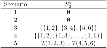
The error variance σ2 was chosen to achieve a signal-to-noise ratio (SNR) of either 2 or 3. The set of main effects in S∗, S1∗, was 1, . . . ,10. The subset of variables involved in interactions was 1, . . . ,6. The set of first-order interactions in S∗ chosen in the different scenarios, S2∗, is displayed in Table 1, and we tookS∗ =S1∗∪S2∗ soS∗ contained no higher order interactions. In each simulation run,β∗S∗
1 was fixed and given by
Scenario S2∗
1 ∅
2 ∅
3 {{1,2},{3,4},{5,6}} 4 {{1,2},{1,3}, . . . ,{1,6}} 5 I(1,2,3)∪ I(4,5,6)
Table 1: Simulation settings.
Each component of β∗S∗
2 was chosen to be q
kβ∗S∗ 1k
2
2/|S1∗|. Thus the squared magnitude of
the interactions was equal to average of the squared magnitudes of the main effects. In all of the scenarios, we applied four methods: the Lasso using only the main effects; iterated Lasso fits; marginal screening for interactions followed by the Lasso; and the Lasso with Backtracking. Note that due to the size ofpin these examples, most of the methods for finding interactions in lower-dimensional data discussed in Section 1, are computationally impractical here.
For the iterated Lasso fits, we repeated the following process. Given a design matrix, first fit the Lasso. Then apply 5-fold cross-validation to give aλvalue and associated active set. Finally add all interactions between variables in this active set to the design matrix, ready for the next iteration. For computational feasibility, the procedure was terminated when the number of variables in the design matrix exceededp+ 250×249/2.
With the marginal screening approach, we selected the 2p interactions with the largest marginal correlation with the response and added them to the design matrix. Then a regular Lasso was performed on the augmented matrix of predictors.
Additionally, in scenarios 3–5, we applied the Lasso with all main effects and only the true interactions. This theoretical Oracle approach provided a gold standard against which to test the performance of Backtracking.
We used the procedures mentioned to yield active sets on which we applied OLS to give a final estimator. To select the tuning parameters of the methods we used cross-validation randomly selection 5 folds but repeating this a total of 5 times to reduce the variance of the cross-validation scores. Thus for each λ value we obtained an estimate of the expected prediction error that was an average over the observed prediction errors on 25 (overlapping) validation sets of size n/5 = 50. Note that for both Backtracking and the iterated Lasso, this form of cross-validation chose not just aλ value but also a path rank. When using Backtracking, the size of the active set was restricted to 50 and the size of Ck
top+ 50×49/2 = 1225, so T was at most 50.
In scenarios 1 and 2, the results of the methods were almost indistinguishable except that the screening approach performed far worse in scenario 1 where it tended to select several false interactions which in turn hampered the selection of main effects and resulted in a much larger prediction error.
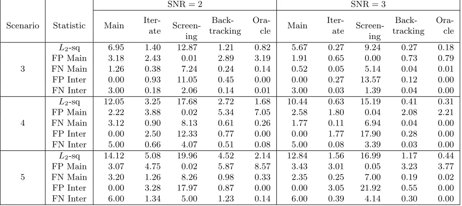
The results of scenarios 3–5, where the signal contains interactions, are more interesting and given in Table 2. For each scenario, method and SNR level, we report 5 statistics. ‘L2
on training data (Ytrain,Xtrain), evaluated at a random independent test observation xnew:
Exnew,Ytrain,Xtrain(f ∗{x
new)−ˆf(xnew;Ytrain,Xtrain)}2.
‘FP Main’ and ‘FP Inter’ are the numbers of noise main effects and noise interaction terms respectively, incorrectly included in the final active set. ‘FN Main’ and ‘FN Inter’ are the numbers of true main effects and interaction terms respectively, incorrectly excluded from the final active set.
For all the statistics presented, lower numbers are to be preferred. However, the higher number of false selections incurred by both Backtracking and the Oracle procedure com-pared to using the main effects only or iterated Lasso fits, is due to the model selection criterion being the expected prediction error. It should not be taken as an indication that the latter procedures are performing better in these cases.
Backtracking performs best out of the four methods compared here. Note that under all of the settings, iterated Lasso fits incorrectly selects more interaction terms than Backtrack-ing. We see that the more careful way in which Backtracking adds candidate interactions, helps here. Unsurprisingly, fitting the Lasso on just the main effects performs rather poorly in terms of predictive performance. However, it also fails to select important main effects; Backtracking and Iterates have much lower main effect false negatives. The screening ap-proach appears to perform worst here. This is partly because it is not making use of the fact that in all of the examples considered, the main effects involved in interactions are also informative. However, its poor performance is also due the fact that too many false interactions are added to the design matrix after the screening stage. Reducing the number added may help to improve results, but choosing the number of interactions to include via cross-validation, for example, would be computationally costly, unless a Backtracking-type strategy of the sort introduced in this paper were used. We also note that for very large
p, marginal screening of interactions would be infeasible due to the quadratic scaling in complexity withp.
5.2 Data Analyses
In this section, we look at the performance of Backtracking using two base procedures, the Lasso for the linear model and the Lasso for multinomial regression, on a regression and a classification data set. As competing methods, we consider simply using the base procedures (‘Main’), iterated Lasso fits (‘Iterated’), Lasso following marginal screening for interactions (‘Screening’), Random Forests (Breiman, 2001), hierNet (Bien et al., 2013) and MARS (Friedman, 1991) (implemented using Hastie et al. (2013)). Note that we do not view the latter two methods as competitors of Backtracking, as they are designed for use on lower dimensional data sets than Backtracking is capable of handling. However, it is still interesting to see how the methods perform on data of dimension that is perhaps approaching the upper end of what is easily manageable for methods such as hierNet and MARS, but at the lower end of what one might use Backtracking on.
SNR = 2 SNR = 3
Scenario Statistic Main
Iter-ate Screen-ing
Back-tracking
Ora-cle Main
Iter-ate Screen-ing
Back-tracking
Ora-cle
3
L2-sq 6.95 1.40 12.87 1.21 0.82 5.67 0.27 9.24 0.27 0.18 FP Main 3.18 2.43 0.01 2.89 3.19 1.91 0.65 0.00 0.73 0.79 FN Main 1.26 0.38 7.24 0.24 0.14 0.52 0.05 5.14 0.04 0.01 FP Inter 0.00 0.93 11.05 0.45 0.00 0.00 0.27 13.57 0.12 0.00 FN Inter 3.00 0.18 2.06 0.14 0.01 3.00 0.03 1.39 0.04 0.00
4
L2-sq 12.05 3.25 17.68 2.72 1.68 10.44 0.63 15.19 0.41 0.31 FP Main 2.22 3.88 0.02 5.34 7.05 2.58 1.80 0.04 2.08 2.21 FN Main 3.12 0.90 8.13 0.61 0.26 1.77 0.11 6.94 0.04 0.00 FP Inter 0.00 2.50 12.33 0.77 0.00 0.00 1.77 17.90 0.28 0.00 FN Inter 5.00 0.66 4.07 0.51 0.08 5.00 0.08 3.39 0.03 0.00
5
L2-sq 14.12 5.08 19.96 4.52 2.14 12.84 1.56 16.99 1.17 0.44 FP Main 3.07 4.75 0.02 5.87 8.57 3.43 3.01 0.05 3.23 3.77 FN Main 3.20 1.26 8.26 0.98 0.33 2.35 0.25 7.00 0.19 0.02 FP Inter 0.00 3.28 17.97 0.87 0.00 0.00 3.05 21.92 0.55 0.00 FN Inter 6.00 1.34 5.00 1.23 0.14 6.00 0.39 4.14 0.30 0.00
Table 2: Simulation results.
5.2.1 Communities and Crime
This data set available athttp://archive.ics.uci.edu/ml/datasets/Communities+and+ Crime+Unnormalized contains crime statistics for the year 1995 obtained from FBI data, and national census data from 1990, for various towns and communities around the USA. We took violent crimes per capita as our response: violent crime being defined as murder, rape, robbery, or assault. The data set contains two different estimates of the populations of the communities: those from the 1990 census and those from the FBI database in 1995. The latter was used to calculate our desired response using the number of cases of violent crimes. However, in several cases, the FBI population data seemed suspect and we discarded all observations where the maximum of the ratios of the two available population estimates differed by more than 1.25. In addition, we removed all observations that were missing a response and several variables for which the majority of values were missing. This resulted in a data set with n= 1903 observations and p= 101 covariates. The response was scaled to have empirical variance 1.
5.2.2 ISOLET
5.3 Methods and Results
For the Communities and crime data set, we used the Lasso for the linear model as the base regression procedure for Backtracking and Iterates. Since the per capita violent crime response was always non-negative, the positive part of the fitted values was taken. For Main, Backtracking, Iterates, Screening and hierNet, we employed 5-fold cross-validation with squared error loss to select tuning parameters. For MARS we used the default settings for pruning the final fits using generalised cross-validation. With Random Forests, we used the default settings on both data sets. For the classification example, penalised multinomial regression was used (see Section 4.1) as the base procedure for Backtracking and Iterates, and the deviance was used as the loss function for 5-fold cross-validation. In all of the methods except Random Forests, we only included first-order interactions. When using Backtracking, we also restricted the size ofCk top+ 50×49/2 =p+ 1225.
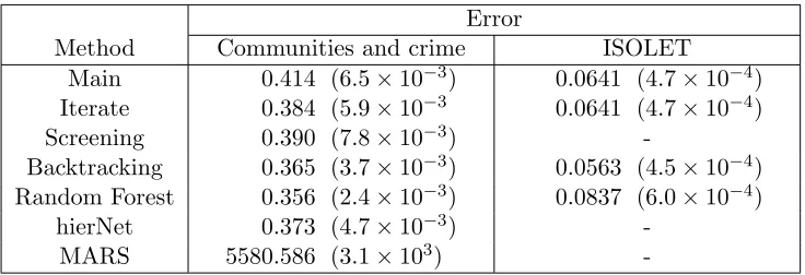
To evaluate the procedures, we randomly selected 2/3 for training and the remaining 1/3 was used for testing. This was repeated 200 times for each of the data sets. Note that we have specifically chosen data sets with nlarge as well as plarge. This is to ensure that comparisons between the performances of the methods can be made with more accuracy. For the regression example, out-of-sample squared prediction error was used as a measure of error; for the classification example, we used out-of-sample misclassification error with 0–1 loss. The results are given in Table 3.
Random Forests has the lowest prediction error on the regression data set, with Back-tracking not far behind, whilst BackBack-tracking wins in the classification task, and in fact achieves strictly lower misclassification error than all the other methods on 90% of all test samples. Note that a direct comparison with Random Forests is perhaps unfair, as the latter is a black-box procedure whereas Backtracking is aiming for a more interpretable model.
MARS performs very poorly indeed on the regression data set. The enormous prediction error is caused by the fact that whenever observations corresponding to either New York or Los Angeles were in the test set, MARS predicted their responses to be far larger than they were. However, even with these observations removed, the instability of MARS meant that it was unable to give much better predictions than an intercept-only model.
HierNet performs well on this data set, though it is worth noting that we had to scale the interactions to have the same`2-norm as the main effects to get such good results (the default
scaling produced error rates worse than that of an intercept-only model). Backtracking does better here. One reason for this is that the because the main effects are reasonably strong in this case, a low amount of penalisation works well. However, because with hierNet, the penalty on the interactions is coupled with the penalty on the main effects, the final model tended to include close to two hundred interaction terms. The Screening approach similarly suffers from including too many interactions and performs only a little better than a main effects only fit.
Error
Method Communities and crime ISOLET
Main 000000.414 (6.5×10⁻³) 00000.0641 (4.7×10⁻⁴) Iterate 000000.384 (5.9×10⁻³ 00000.0641 (4.7×10⁻⁴)
Screening 000000.390 (7.8×10⁻³)
-Backtracking 000000.365 (3.7×10⁻³) 00000.0563 (4.5×10⁻⁴) Random Forest 000000.356 (2.4×10⁻³) 00000.0837 (6.0×10⁻⁴)
hierNet 000000.373 (4.7×10⁻³)
-MARS 005580.586 (3.1×10³)
-Table 3: Real data analyses results. Average error rates over 200 training–testing splits are given, with standard deviations of the results divided by√200 in parentheses.
by Backtracking. This occurs in a rather extreme way with the ISOLET data set where, since in the first stage of the iterated Lasso, cross-validation selected far too many variables (>250), the second and subsequent steps could not be performed. This is why the results are identical to using the main effects alone.
6. Theoretical Properties
Our goal in this section is to understand under what circumstances Backtracking with the Lasso can arrive at a set of candidates, C∗, that contains all of the true interactions, and only a few false interactions. On the event on which this occurs, we can then apply many of the existing results on the Lasso, to show that the solution path ˆβ(λ, C∗) has certain properties. As an example, in Section 6.2 we give sufficient conditions for the existence of a λ∗ such that{v: ˆβv(λ∗, C∗)6= 0}equals the true set of variables.
We work with the normal linear model with interactions,
Y=µ∗1+XS∗β∗S∗+ε, (7)
where εi i.∼i.d. N(0, σ2), and to ensure identifiability, XS∗ has full column rank. We will
assume that S∗ = S1∗ ∪S2∗, where S1∗ and S2∗ are main effects and two-way interactions respectively. Let the interacting main effects be I∗; formally, I∗ is the smallest set of main effects such thatI(I∗)⊇S2∗. Assume I∗ ⊆S1∗ so interactions only involve important main effects. Let sl =|Sl∗|,l= 1,2 and set s=s1+s2. Define C∗ =C1∪ I(S1∗). Note that C∗
containsS∗ but not additional interactions from any variables fromC1\S1∗.
Although the Backtracking algorithm was presented for a base path algorithm that computed solutions at only discrete values, for the following results, we need to imagine an idealised algorithm which computes the entire path of solutions. In addition, we will assume that we only allow first-order interactions in the Backtracking algorithm, and that
T ≥s1.
6.1 Random Normal Design
Let the random matrixZhave independent rows distributed asNp(0,Σ). Suppose thatXC1,
the matrix of main effects, is formed by scaling and centringZ. We consider an asymptotic regime where X, f∗, S∗, σ2 and p can all change as n → ∞, though we will suppress their dependence onn in the notation. Furthermore, for sets of indices S, M ⊆ {1, . . . , p}, let ΣS,M ∈ R|S|×|M| denote the submatrix of Σ formed from those rows and columns of Σ indexed by S and M respectively. For any positive semi-definite matrix A, we will let cmin(A) and cmax(A) denote its minimal and maximal eigenvalues respectively. For
sequencesan,bn, by anbnwe mean bn=o(an). We make the following assumptions.
A1. cmin(ΣS∗1,S1∗)≥c∗ >0.
A2. supτ∈Rs1:kτk∞≤1kΣN,S∗ 1Σ
−1
S1∗,S∗1τk∞≤δ <1.
A3. s41log(p)/n→0 ands81log(s1)2/n→0.
A4.
min
j∈I∗|β ∗ j|
s1(σ
√
logp√+√s1+ logp)
n +
p
s31log(s1) n1/3 .
A5. kβ∗S∗
2k2 is bounded asn→ ∞and cmax(ΣS ∗
1,S∗1)≤c ∗<∞.
A1 is a standard assumption in high-dimensional regression and is, for example, implied by the compatibility constant of B¨uhlmann and van de Geer (2011a) being bounded away from zero. A2 is closely related to irrepresentable conditions (see Meinshausen and B¨uhlmann (2006), Zhao and Yu (2006), Zou (2006), B¨uhlmann and van de Geer (2011a), Wainwright (2009)), which are used for proving variable selection consistency of the Lasso. Note that although here the signal may contain interactions, our irrepresentable-type condition only involves main effects.
A3 places restrictions on the rates at whichs1 andpcan increase withn. The first con-dition involving log(p) is somewhat natural ass21log(p)/n→0 would typically be required in order to show`1 estimation consistency ofβ where onlys1 main effects are present; here our effective number of variables is s1 ≤s≤s21. The second condition restricts the size of
s1more stringently but is nevertheless weaker than equivalent conditions in Hao and Zhang
(2014).
A4 is a minimal signal strength condition. The term involving σ is the usual bound on the signal strength required in results on variable selection consistency with the Lasso when there are s2
1 non-zero variables. Due to the presence of interactions, the terms not
involving σ place additional restrictions on the sizes of non-zero components of β∗ even when σ= 0. A5 ensures that the model is not too heavily misspecified in the initial stages of the algorithm, where we are regressing on only main effects.
The following theorem states that given the assumptions above, with probability tending to 1 we are guaranteed a candidate set will be produced by our algorithm which contains all true interactions and no interactions involving a noise variable.
6.2 Fixed Design
The result for a random normal design above is based on a corresponding result for fixed design which we present here. In order for Backtracking not to add any interactions involving noise variables, to begin with, one pair of interacting signal variables must enter the solution path before any noise variables. Other interacting signal variables need only become active after the interaction between this first pair has become active. Thus we need that there is some ordering of the interacting variables where each variable only requires interactions between those variables earlier in the order to be present before it can become active. Variables early on in the order must have the ability to be selected when there is serious model misspecification as few interaction terms will be available for selection. Variables later in the order only need to have the ability to be selected when the model is approximately correct.
Note that a signal variable having a coefficient large in absolute value does not necessarily ensure that it becomes active before any noise variable. Indeed, in our example in Section 2, variable 5 did not enter the solution path at all when only main effects were present, but had the largest coefficient. Write f∗ for XS∗βS∗, and for a set S such that XS has full
column rank, define
βS:= (XTSXS)−1XTSf∗.
Intuitively what should matter are the sizes of the appropriate coefficients ofβSfor suitable choices ofS. In the next section, we give a sufficient condition based on βS for a variable
v∈S to enter the solution path before any variable outside S.
6.2.1 The Entry Condition
Let PS = X
S(XTSXS)−1XTS denote orthogonal projection on to the space spanned by
the columns of XS. Further, for any two candidate sets S, M that are sets of subsets
of {1, . . . , p}, define
ˆ
ΣS,M = n1XTSXM.
Now given a set of candidates,C, let v∈S ⊂C and write M =C\S. Forη >0, we shall say that the Ent(v, S, C;η) condition holds if,XS has full column rank, and the following
holds,
sup
τS∈R|S|:kτSk∞≤1
kΣˆM,SΣˆ −1
S,SτSk∞<1, (8)
|βvS|>max
u∈M (1
n
XTu(I−PS)f∗ + 2η
1− kΣˆ−1S,SΣˆS,{u}k1
+η )
k( ˆΣ−1S,S)vk1. (9)
In Lemma 4 given in the appendix, we show that this condition is sufficient for variable
v to enter the active set before any variable in M, when the set of candidates is C and kXT
Cεk∞≤η. In addition, we show that v will remain in the active set at least until some
variable fromM enters the active set.
1 nX
T
u(I−PS)f∗ term is the sample covariance between Xu, which is one of the columns of XM, and the residual from regressing f∗ onXS. Note that the more ofS∗ thatS contains,
the closer this will be to 0.
To understand the k( ˆΣ−1S,S)vk1 term, without loss of generality take v as{1}and write b = ˆΣS\{v},{v} and D = ˆΣS\{v},S\{v}. For any square matrix ˆΣ, let cmin( ˆΣ) denote its
minimal eigenvalue. Using the formula for the inverse of a block matrix and writing sfor |S|, we have
k( ˆΣ−1S,S)vk1 =
1 +bT(D−bbT)−1b
−(D−bbT)−1b
1
≤1 +kbk
2 2+
√
s−1kbk2 cmin( ˆΣS,S)
.
In the final line we have used the Cauchy–Schwarz inequality and the fact that if w∗ is a unit eigenvector ofD−bbT with minimal eigenvalue, then
cmin(D−bbT) =
ˆ
ΣS,S
−bTw∗ w∗
2
≥cmin( ˆΣS,S) q
1 +|bTw∗|2 ≥c
min( ˆΣS,S).
Thus when variable v is not too correlated with the other variables in S, and so kbk2 is small, k( ˆΣ−1S,S)vk1 will not be too large. Even when this is not the case, we still have the
bound
k( ˆΣ−1S,S)vk1≤ p
|S|
cmin( ˆΣS,S) .
Turning now to the denominator, kΣˆ−1S,SΣˆS,{u}k1 is the `1-norm of the coefficient of
regression ofXu onXS, and the maximum of this quantity overu∈M gives the left-hand
side of (8). Thus whenuis highly correlated with many of the variables inS,kΣˆS,S−1ΣˆS,{u}k1
will be large. On the other hand, in this case one would expect k(I−PS)Xuk2 to be small,
and so to some extent the numerator and denominator compensate for each other.
6.2.2 Statement of Results
Without loss of generality assume I∗ = {1, . . . ,|I∗|}. Also let J = {I(A) : A ⊆ S1∗}. Our formal assumption corresponding to the discussion at the beginning of Section 6 is the following.
The entry order condition. There is some ordering of the variables in I∗, which without loss of generality we take to simply be 1, . . . ,|I∗|, such that for each j∈I∗, we have,
For allA∈ J with I(1, . . . , j−1)⊆A⊆ I(S1∗) Ent(j, S1∗∪B, C1∪A;η) holds for someA∩S2∗⊆B⊆A.
Here
η=η(t;n, p, s1, σ) =σ r
t2+ 2 log(p+s2 1)
First we discuss the implications for variable 1. The condition ensures that whenever the candidate set is enlarged from C1 to also include any set of interactions built from S1∗,
variable 1 enters the active set before any variable outsideI(S1∗), and moreover, it remains in the active set at least until a variable outside I(S1∗) enters.
For j > 2, we see that the enlarged candidate sets for which we require the entry conditions to hold, are fewer in number. Variable |I∗|only requires the entry condition to hold for candidate sets that at least includeI(1, . . . ,|I∗| −1) and thus include almost all of
S∗. What this means is that we require some ‘strong’ interacting variables, for which when
f∗is regressed onto a variety of sets of variables containing them (some of which contain only a few of the true interaction variables), always have large coefficients. Given the existence of such strong variables, other interacting variables need only have large coefficients whenf∗ is regressed onto sets containing them that also include many true interaction terms. Note that the equivalent result for the success of the strategy that simply adds interactions between selected main effects would essentially require all main effect involved in interactions to satisfy the conditions imposed on the variables 1 and 2 here. Going back to the example in Section 2, variable 5 has |β5S| ≈0 for all S ⊆ {1, . . . ,6}, but |β5S|>0 once{1,2} ∈S or {3,4} ∈S.
Theorem 2 Assume the entry order condition holds. With probability at least1−exp(−t2/2), there exists a k∗ such thatC∗ ⊇Ck∗ ⊇S∗.
The following corollary establishes variable selection consistency under some additional conditions.
Corollary 3 Assume the entry order condition holds. WritingN =C∗\S∗, further assume
kΣˆN,S∗Σˆ −1
S∗,S∗sgn(β∗S∗)k∞<1;
and that for all v∈S∗,
|β∗v|> η
sgn(β
∗ S∗)T( ˆΣ
−1 S∗,S∗)v
1− kΣˆN,S∗Σˆ −1
S∗,S∗sgn(β∗S∗)k∞
+ξ,
where
ξ=ξ(t;n, s, σ, cmin( ˆΣS∗,S∗)) =σ s
t2+ 2 log(s) ncmin( ˆΣS∗,S∗)
.
Then with probability at least 1−3 exp(−t2/2), there exist k∗ andλ∗ such that
A( ˜β(λ∗, Ck∗)) =S∗.
Note that if we were to simply apply the Lasso to the set of candidates Call := C1 ∪ I(C1) (i.e. all possible main effects and their first-order interactions), we would require an
irrepresentable condition of the form kΣˆNall,S∗Σˆ
−1
S∗,S∗sgn(β∗S∗)k∞<1,
where Nall = Call \S∗. Thus we would need O(p2) inequalities to hold, rather than our
7. Discussion
While several methods now exist for fitting interactions in moderate-dimensional situations wherep is in the order of hundreds, the problem of fitting interactions when the data is of truly high dimension has received less attention.
Typically, the search for interactions must be restricted by first fitting a model using only main effects, and then including interactions between those selected main effects, as well as the original main effects, as candidates in a final fit. This approach has the drawbacks that important main effects may not be selected in the initial stage as they require certain interactions to be present in order for them to be useful for prediction. In addition, the initial model may contain too many main effects when, without the relevant interactions, the model selection procedure cannot find a good sparse approximation to the true model. The Backtracking method proposed in this paper allows interactions to be added in a more natural gradual fashion, so there is a better chance of having a model which contains the right interactions. The method is computationally efficient, and our numerical results demonstrate its effectiveness for both variable selection and prediction.
From a theoretical point of view we have shown that when used with the Lasso, rather than requiring all main effects involved in interactions to be highly correlated with the signal, Backtracking only needs there to exist some ordering of these variables where those early on in the order are important for predicting the response by themselves. Variables later in the order only need to be helpful for predicting the response when interactions between variables early on in the order are present.
Though in this paper, we have largely focussed on Backtracking used with the Lasso, the method is very general and can be used with many procedures that involve sparsity-inducing penalty functions. These methods tend to be some of the most useful for dealing with high-dimensional data, as they can produce stable, interpretable models. Combined with Backtracking, the methods become much more flexible, and it would be very inter-esting to explore to what extent using non-linear base procedures could yield interpretable models with predictive power comparable to black-box procedures such as Random Forests (Breiman, 2001). In addition, we believe integrating Backtracking with some of the penalty-based methods for fitting interactions to moderate-dimensional data, will prove to be a fruitful direction for future research.
Acknowledgments
I am very grateful to Richard Samworth, for many helpful comments and suggestions.
Appendix A. Construction of X in Section 2
First, consider (Zi1, Zi2, Zi3) generated from a mean zero multivariate normal distribution
with Var(Zij) = 1,j = 1,2,3, Cov(Zi1, Zi2) = 0 and Cov(Zi1, Zi3) = Cov(Zi2, Zi3) = 1/2.
probability 1/2. We form theith row of the design matrix as follows:
Xi1 =Ri1sgn(Zi1)|Zi1|1/4, Xi2 =Ri1|Zi1|3/4,
Xi3 =Ri2sgn(Zi2)|Zi2|1/4, Xi4 =Ri2|Zi2|3/4,
Xi5 =Zi3.
The remaining Xij, j = 6, . . . , pare independently generated from a standard normal
dis-tribution. Note that the random signs Ri1 and Ri2 ensure that Xi5 is uncorrelated with
each of Xi1, . . . , Xi4. Furthermore, the fact that Xi1Xi2 = Zi1 and Xi3Xi4 = Zi2, means
that whenβ5 =−12(β7+β8),Xi5 is uncorrelated with the response. Appendix B. Proofs of Theorem 2 and Corollory 3
In this subsection we use many ideas from Section B of Wainwright (2009) and Section 6 of B¨uhlmann and van de Geer (2011a).
Lemma 4 Let S ⊆ C be such that XS has full column rank and let M =C\S. On the
event
ΩC,η:={n1kXTCεk∞≤η},
the following hold:
(i) If
λ >max
u∈M (1
n|XTu(I−PS)f∗|+ 2η
1− kΣˆ−1S,SΣˆS,{u}k1 )
, (10)
then the Lasso solution is unique and βˆM(λ, C) =0.
(ii) Ifλ is such that for some Lasso solutionβˆM(λ, C) =0, and for v∈S,
|βvS|>k( ˆΣS,S−1)vk1(λ+η),
then for all Lasso solutions, βˆv(λ, C)6= 0.
(iii) Let
λent = sup{λ:λ≥0 and for some Lasso solution βˆM(λ, C)6=0},
where we take sup∅= 0. If for v∈S,
|βvS|>max
u∈M (1
n|X T
u(I−PS)f∗|+ 2η
1− kΣˆ−1S,SΣˆS,{u}k1
+η )
k( ˆΣ−1S,S)vk1,
there exists aλ > λent such that the solutionβˆ(λ, C)is unique, and for allλ0 ∈(λent, λ]
Proof We begin by proving (i). Suppressing the dependence of ˆβ on λ and C, we can write the KKT conditions ((3), (4)) as
1
nX T
C(Y−XCβˆ) =λτˆ,
where ˆτ is an element of the subdifferential ∂kβˆk1 and thus satisfies
kτˆk∞≤1, (11)
ˆ
βv 6= 0⇒τˆv = sgn( ˆβv). (12)
By decomposingYasPSf∗+(I−PS)f∗+ε,XC as (XSXM), and noting thatXTS(I−PS) = 0, we can rewrite the KKT conditions in the following way:
1 nX
T S(PSf
∗−
XSβˆS) +n1X T
Sε−ΣˆS,MβˆJ∗ =λτˆS, (13) 1
nX T
M(PSf∗−XSβˆS) +n1X T
M{(I−PS)f∗+ε} −ΣˆM,MβˆM =λτˆM. (14)
Now let ˘βS be a solution to the restricted Lasso problem,
(ˆµ,β˘S) = arg min
µ,βS
1
2nkY−µ1−XSβSk2+λkβSk1 .
The KKT conditions give that ˘βS satisfies 1
nX T
S(Y−XSβ˘S) =λτ˘S, (15)
where ˘τS ∈∂kβ˘Sk1. We now claim that
( ˆβS,βˆM) = ( ˘βS,0) (16)
(ˆτS,τˆM) =
˘
τS,ΣˆM,SΣˆ −1
S,S(˘τS−1nλ−1XTSε) +1nλ −1XT
M{(I−PS)f∗+ε}
(17)
is the unique solution to (13), (14), (11) and (12). Indeed, as ˘βS solves the reduced Lasso problem, we must have that (13) and (12) are satisfied. Multiplying (13) byXSΣˆ
−1
S,S, setting
ˆ
βM =0 and rearranging gives us that
PSf∗−XSβˆS =XSΣˆ −1
S,S(λτˆS−n1XTSε), (18)
and substituting this into (14) shows that our choice of ˆτM satisfies (14). It remains to
check that we havekτˆMk∞≤1. In fact, we shall show that kτˆMk∞<1. Since we are on
ΩC,η andkτ˘Sk∞≤1, foru∈M we have
λ|τˆu| ≤ kΣˆ −1
S,SΣˆS,{u}k1 λkτ˘Sk∞+k1nXTSεk∞+1n
XTu(I−PS)f∗+n1 XTuε < λkΣˆ−1S,SΣˆS,{u}k1+n1
where the final inequality follows from (10). We have shown that there exists a solution, ˆβ, to the Lasso optimisation problem with ˆβM = 0. The uniqueness of this solution follows from noting that kτˆMk∞ < 1, XS has full column rank and appealing to Lemma 1 of
Wainwright (2009).
For (ii), note that from (13), provided ˆβM = 0, we have that
ˆ
βS=βS−Σˆ−1S,S(λτˆS− 1nXTSε).
But by assumption
|βvS|>k( ˆΣS,S−1)vk1(λ+η)≥
( ˆΣ−1S,S)Tv(λτˆS−n1XTSε) ,
whence ˆβv6= 0.
(iii) follows easily from (i) and (ii).
Proof of Theorem 2. In all that follows, we work on the event ΩC∗,η defined in Lemma 4.
Using standard bounds for the tails of Gaussian random variables and the union bound, it is easy to show thatP(Ω1∩ΩC∗,η)≥1−exp(−t2/2). Let N ={1, . . . , p} \S∗
1.
Let ˜T be the number of steps taken by the algorithm: this would typically be T, but may be smaller if a perfect fit is reached or if p < T for example. Let Ck be the largest
member of{C1, . . . , CT˜} satisfying Ck⊆C∗. Such aCk exists sinceC1⊆C∗.
Now suppose for a contradiction that Ck+S∗. Letj be such that
I(1, . . . , j−1)⊆Ck,
withj maximal. Since I(1) =∅, such a j exists. Let A=Ck\C1. Note thatA∈ J and
I(1, . . . , j−1)⊆A⊆C∗\C1 =I(S1∗).
By the entry order condition, we know that j will enter the active set before any variable inN, and before a perfect fit is reached. Thusk+ 1≤T˜ andCk+1 contains only additional
interactions not involving any variables fromN, soCk+1⊆C∗.
Proof of Corollary 3. Let ΩC∗,η be defined as in Lemma 4. Also define the events
Ω1={n1kXTN(I−PS ∗
)εk∞≤η},
Ω2={1nkΣˆ −1
S∗,S∗XTS∗εk∞≤ξ}
In all that follows, we work on the event Ω1∩Ω2∩ΩC∗,η. AsI−PS ∗
is a projection,
P(n1|XvT(I−PS ∗
)ε| ≤η)≥P(n1|XvTε| ≤η).
Further, 1nΣˆ−1S∗,S∗XST∗ε∼N|S∗|(0,1 nσ
2Σˆ−1
whereZ ∼N(0, σ2/(ncmin( ˆΣS∗,S∗))). Note that P(Ω1∩Ω2∩ΩC∗,η)≥1−P(Ωc
C∗,η)−P(Ω1c)−P(Ωc2).
Using this, it is straightforward to show that P(Ω1∩Ω2∩ΩC∗,η)≥1−3 exp(−t2/2).
Since we are on ΩC∗,η, we can assume the existence of ak∗ from Theorem 2. We now
follow the proof of Lemma 4 takingS =S∗ and M =Ck∗\S∗ ⊆N. The KKT conditions
become
ˆ
ΣS∗,S∗(β∗S∗−βˆS∗) +n1XST∗ε−ΣˆS∗,MβˆM =λτˆS∗, (19)
ˆ
ΣM,S∗(β∗
S∗−βˆS∗) +n1XTMε−ΣˆM,MβˆM =λτˆM, (20)
with ˆτ also satisfying (11) and (12) as before. Now let λbe such that
η
1− kΣˆM,S∗Σˆ −1
S∗,S∗sgn(β∗S∗)k∞
< λ < min
v∈S∗
sgn(β
∗ S∗)T( ˆΣ
−1 S∗,S∗)v
−1
(|βv∗| −ξ)
.
It is straightforward to check that ( ˆβS∗,βˆM) = (β∗S∗−λΣˆ
−1
S∗,S∗sgn(β∗S∗) +n1Σˆ −1
S∗,S∗XTS∗ε,0)
(ˆτS∗,τˆM) =
sgn(β∗S∗),ΣˆM,S∗Σˆ −1
S∗,S∗sgn(β∗S∗) +n1λ−1XTM(I−PS ∗
)ε
is the unique solution to (19), (20), (11) and (12).
Appendix C. Proof of Theorem 1
In the following, we make use of notation defined in Section 6.2. In addition, for convenience we write S =S1∗, M =S∪J∗. Also, we will write main effects variables{j} as simply j. For any matrixM,kMk∞will denote maxjk|Mjk|. First we collect together various results
concerning ˆΣC∗,C∗.
Lemma 5 Consider the setup of Theorem 1. LetEnandVarn denote empirical expectation
and variance with respect to Zso that, for example Enzj =Pni=1Zij/n.
(i) Let D be the diagonal matrix indexed by C∗ used to scale transformations of Z in order to create XC∗ i.e. with entries such that D2jj = Varn(zj) and D2vv = Varn(zj− Enzj)(zk−Enzk) whenv={j, k}. Then
max
j∈C1
|Djj2 −1|=OP( p
log(p)/n) (21)
max
{j,k}∈M|D 2
{j,k},{j,k}−1−Σ2jk|=OP( p
log(s1)n−1/4) (22)
(ii)
1 nkX
T
J∗XSk∞=OP( p
log(s1)n−1/3) (23)
cmin( ˆΣS,S)≥c∗−s1OP( p
log(s1)/n) (24)
cmin( ˆΣM,M)≥c2∗+s21OP( p
log(s1)n−1/4) (25) cmax( ˆΣJ∗,J∗)≤2c∗2+s2
1OP( p
Proof We use bounds on the tails of products of normal random variables from Hao and Zhang (2014) (equation B.9). We have
max
j,k |Covn(zj, zk)−Σjk|= maxj,k |En(zjzk)−EnzjEnzk−Σjk|
=OP( p
log(p)/n).
Also, max
j,k,l,m∈S|Covn (zj−Enzj)(zk−Enzk),(zl−Enzl)(zm−Enzm)
−ΣjlΣkm−ΣjmΣkl|
= max
j,k,l,m∈S|En(zjzkzlzm)−En(zjzk)En(zlzk)−ΣjlΣkm−ΣjmΣkl|+OP( p
log(s1)/n)
=OP( p
log(s1)n−1/4).
Now we consider (ii). We have
1 nkX
T
J∗XSk∞≤max v∈J∗D
−1 vv max
k∈S D −1
kk j,k,lmax∈S|Covn (zj−Enzj)(zk−Enzk), zl
|
≤OP( p
log(s1)n−1/3),
the rate being driven by the size of En(zjzkzl). Also
cmin( ˆΣS,S) = min τ∈Rs1:kτk
2=1
τ{ΣS,S−(ΣS,S−ΣˆS,S)}τ
≥cmin(ΣS,S)− max
τ∈Rs1:kτk2=1kτk
2
1kΣS,S−ΣˆS,Sk∞
=c∗−s1OP( p
log(s1)/n).
Now let ˜Σbe a matrix with entries indexed byM with ˜
Σuv= ΣjlΣkm+ ΣjmΣkl
whenu={j, k}andv={l, m}. Lemma A.4 of Hao and Zhang (2014) shows thatcmin( ˜Σ)≥
2cmin(ΣS,S)2 and cmax( ˜Σ)≤2cmax(ΣS,S)2. Thus we have cmin( ˆΣM,M) = min
τ∈R|M|:kDM,Mτk2=1
τDM,MΣˆM,MDM,Mτ
≥ kDM,Mk−1∞cmin(DM,MΣˆM,MDM,M)
≥ {1 +OP( p
log(s1)n−1/4)}[c2∗−s21{kΣ˜ −DM,MΣˆM,MDM,M)k∞+OP( p
log(s1)n−1/3)}] ≥c2∗+s21OP(
p
log(s1)n−1/4).
Similarly
cmax( ˆΣJ∗,J∗) = max
τ∈R|J∗|:kDJ∗,J∗τk2=1
τDJ∗,J∗ΣˆJ∗,J∗DJ∗,J∗τ
≤ {1−OP( p
log(s1)n−1/4)}cmax(DJ∗,J∗ΣˆJ∗,J∗DJ∗,J∗)
≤ {1−OP( p
log(s1)n−1/4)}{2c∗2+s21kΣ˜ −DJ∗,J∗ΣˆJ∗,J∗DJ∗,J∗)k∞}
≤2c∗2+s21OP( p
Lemma 6 Working with the assumptions of Theorem 1, we have
max
A∈J kβ S∪A
S −β∗Sk∞≤OP( q
s3
1log(s1)n−1/3). Proof For A ∈ J let ∆A ∈ R|S∪A| with ∆A
S = βS ∪A
S −β∗S and ∆AA = βS ∪A
A . Define g∗=XS∗
2β ∗
S∗2. Note that
f∗=XSβ∗S+g ∗,
so
∆A= (XTS∪AXS∪A)−1XS∪Ag∗.
First we boundk∆AAk2
2 in terms of kg∗k22. We have that
kXS∪A∆Ak22 =kXS∆ASk22+ 2∆AS T
XTSXA∆AA+kXA∆AAk22≤ kg∗k22.
Thus
cmin(n1XTSXS)k∆ASk22−2 p
|A||S|k1nXTSXAk∞k∆AAk2k∆ASk2+cmin(n1XTAXA)k∆AAk22−n1kg ∗k2
2 ≤0.
Thinking of this as a quadratic ink∆ASk2 and considering the discriminant yields k∆AAk22≤
1 ncmin(
1
nXTSXS)kg∗k22
cmin(1nXTSXS)cmin(n1XTAXA)− kn1XTSXAk2∞|A||S| .
Thus by Lemma 5 (ii) and condition A2, maxA∈Jk∆AAk2= √1nkg∗k2OP(1).
But
1 √
nkg ∗k
2≤ q
cmax( ˆΣJ∗,J∗)kβ∗
S2∗k2=OP(1)
by Lemma 5 (ii) and A5, so maxA∈J k∆AAk2 =OP(1).
Next observe that
kXS∪A∆A−g∗k22 ≤ kXA∆AA−g∗k22,
so
k∆ASk22cmin(1nXTSXS)≤ 1nkXS∆ASk22
≤2|n1∆ASTXTS(XA∆AA−g ∗)|
≤2p|A||S|k∆SAk2kn1XTSXAk∞k∆AAk2+ 2k∆ASk2k1nXTSg ∗k
2.
Therefore
k∆ASk∞≤2{cmin(n1XTSXS)}−1( p
|A||S|k1 nX
T
SXAk∞k∆AAk2+kn1XTSg∗k2),
so
max
A∈J k∆ A
Sk∞≤2{cmin(n1XTSXS)}−1( p
|S||J∗|k1 nX
T
SXJ∗k∞OP(1) +k1 nX
Now
kn1XTSg∗k2 ≤
√
s1kn1XTSXS∗2k∞kβ ∗ S∗2k1
≤OP(s1 p
log(s1)n−1/3).
Thus
max
A∈J k∆ A
Sk∞≤OP( q
s3
1log(s1)n−1/3).
Proof of Theorem 1. In view of Theorem 2 and its proof, it is enough to show that with probability tending to 1, we have
max
A∈J τsup∈Rs1
kΣˆN,S∪AΣˆ −1
S∪A,S∪Aτk∞<1, (27)
min
j∈I∗Amin∈J|β S∪A
j |>max A∈J maxj∈N
1 n|X
T
j(I−PS∪A)f∗|+ 2n1kX T C∗εk∞
1− kΣˆ−1S∪A,S∪AΣˆS∪A,jk1
+n1kXTC∗εk∞
p
|M|
cmin( ˆΣM,M) .
(28)
First note that for j ∈ N, Zj = ZSΣS,S−1ΣS,j +Ej where Ej is independent of ZS and Ej ∼Nn(0,(1−Σj,SΣ−1S,SΣS,j)I). Thus
XjDjj=XSDS,SΣS,S−1ΣS,j +Ej−1E¯j,
and
max
A∈J k(X T
S∪AXS∪A)−1XTS∪AXjk1≤Dkk−1kDS,SΣ−1S,SΣS,jk1+ max A∈J k
ˆ
Σ−1S∪A,S∪An1X T
S∪AEjk1.
Now the second term above is at most
max
A∈J τ∈R|Smax∪A|:kτk2≤1
kΣˆ−1S∪A,S∪Aτk1k1nXTMEjk2.
But
max
A∈J τ∈R|S∪maxA|:kτk∞≤1k
ˆ
Σ−1S∪A,S∪Aτk1 ≤ p
|M|
cmin( ˆΣM,M)
≤
p
|M|
c2
∗+s21OP( p
log(s1)n−1/4).
Also since forv∈M andj ∈N,XTvEj/n∼N(0,1) we have
max
j∈N k 1 nX
T
MEjk22 ≤ |M|OP(log(p)/n).
Therefore
max
A∈J τsup∈ Rs1
kΣˆN,S∪AΣˆ −1
S∪A,S∪Aτk∞≤(1 +oP(1))δ+
s21oP(1) c2