On Robustness Properties of Convex Risk Minimization Methods for
Pattern Recognition
Andreas Christmann [email protected] University of Dortmund
Department of Statistics 44221 Dortmund, Germany
Ingo Steinwart [email protected]
Modeling, Algorithms and Informatics Group, CCS-3 Mail Stop B256
Los Alamos National Laboratory Los Alamos, NM 87545, USA
Editor: Peter Bartlett
Abstract
The paper brings together methods from two disciplines: machine learning theory and robust statis-tics. We argue that robustness is an important aspect and we show that many existing machine learning methods based on the convex risk minimization principle have−besides other good prop-erties−also the advantage of being robust. Robustness properties of machine learning methods based on convex risk minimization are investigated for the problem of pattern recognition. As-sumptions are given for the existence of the influence function of the classifiers and for bounds on the influence function. Kernel logistic regression, support vector machines, least squares and the AdaBoost loss function are treated as special cases. Some results on the robustness of such methods are also obtained for the sensitivity curve and the maxbias, which are two other robustness criteria. A sensitivity analysis of the support vector machine is given.
Keywords: AdaBoost loss function, influence function, kernel logistic regression, robustness, sensitivity curve, statistical learning, support vector machine, total variation
1. Introduction
In statistical learning theory the principle of regularized empirical risk minimization based on con-vex loss functions plays an important role, see Vapnik (1998). One strong argument in favor of such methods is that many classifiers based on convex loss functions are universally consistent under weak conditions. Nevertheless, it is important to investigate robustness properties for such statis-tical learning methods for the following reasons. In almost all cases statisstatis-tical models are only approximations to the true random process which generated a given data set and for which a method for analyzing the data is designed. Hence the natural question arises what impact such deviations may have on the results. J.W. Tukey, one of the pioneers of robust statistics, mentioned already in 1960 (Hampel et al., 1986, p. 21):
this hope was often drastically wrong; even mild deviations often have much larger effects than were anticipated by most statisticians.
The main aims of robust statistics are the description of the structure best fitting the bulk of the data and the identification of points deviating from this structure or deviating substructures for further treatment, cf. Hampel et al. (1986). Very briefly, a good robust method can be described as follows.
• If the strict model assumptions are violated, than the results of a robust method are only influenced in a moderate way by a few data points, which deviate grossly from the structure of the bulk of the data set, or by many data points, which deviate only mildly from the structure of the bulk of the data set.
• A robust method should have a reasonable high efficiency when the data set was in fact generated by the assumed model.
In practice one has to apply machine learning methods to a data set with a finite sample size. Ma-chine learning methods are nonparametric tools. Nevertheless, the robustness issue is important, because the classical assumption that all data points were independently generated by the same dis-tribution can be violated in practice. One reason is that outliers often occur in real data sets. Outliers can be described as data points which “are far away. . .from the pattern set by the majority of the data”, see Hampel et al. (1986, p. 25). Sometimes outliers are even correlated, which contradicts the classical assumption that the observations in the data set were generated in an independent manner. There are many reasons for the occurrence of outliers, e.g. typing errors and gross errors, which are errors due to a source of deviations which acts only occasionally but is quite powerful. E.g. undetected outliers may have an extreme impact on the estimation of insurance tariffs computed by motor vehicle insurance companies. From a robustness point of view the occurrence of outliers is only one of several possible deviations from the assumed model. There are often no or virtually no gross errors in high-quality data, but 1% to 10% of gross errors in routine data seem to be more the rule than the exception, cf. Hampel et al. (1986, p. 27f). Especially in large data mining problems the data quality is sometimes far from being optimal, cf. Hand et al. (2001) or Hipp et al. (2001). Obviously, it is not the goal to model the occurrence of typing errors or gross errors, because it is unlikely that they will occur in the same manner for other data sets which will be collected in the future. Goals of robust statistics are to investigate the impact such data points can have on the results of estimation, testing or prediction methods and the development of methods such that the impact of such data points is bounded.
for the next year. Hence, the empirical distribution of the claim amount is in general a mixture of really observed values and of estimated claim amounts. Further, some explanatory variables may have imprecise values. E.g. there is a variable describing how many kilometers a customer is driving with the car within one year. The customer has to choose between some categories, e.g. below 9000 kilometers, between 9000 and 12000 kilometers, between 12000 and 15000 kilometers, and so on. There are reasons making it plausible, that a percentage of these values in the data set are too small,
e.g. it is well-known to the customers that the premium of an insurance tariff increases for increasing
values of this variable. The data set contains data from more than four million customers with more than 70 variables. Hence there is a high probability that some data points are typing errors, although the data set is of high quality.
There are different approaches to robustness in the statistical literature. For statistics repre-sentable as a functional of the empirical distribution, qualitative robustness, which is defined as equicontinuity of the distributions of the statistic as the sample size changes, is closely related to continuity of the statistic viewed as a functional in the weak(-star) topology, cf. Huber (1981, p. 7f) or Hampel et al. (1986, p. 41). The concept of qualitative robustness is a rather weak robustness criterion. It has the disadvantage that it does not offer arguments how to choose among different qualitative robust procedures. Huber’s minimax approach of robust statistics (Huber, 1964, 1981) is to minimize the maximum asymptotic variance of the estimator within a neighborhood of the model. Other strategies of robust statistics are Hampel’s influence function (Hampel, 1974; Hampel et al., 1986), the finite sample breakdown point proposed by Donoho and Huber (1983), the ap-proach based on least favourable local alternatives (Rieder, 1994), and the regression depth method proposed by Rousseeuw and Hubert (1999).
Here, we will mainly use the approach based on the influence function. This approach can be applied to quite general models and the influence function has a nice interpretation, because it is a special Gˆateaux derivative, see Section 3. A map T is called robust in the theory of robust statistics based on influence functions, if T has as a bounded influence function. From the viewpoint of robust statistics it is important to investigate the impact a small amount of contamination of the ‘true’ probability measurePcan have on the statistical learning process which is specified via the regularized theoretical risk, i.e. the objective functions RregL,P,λ(.)and RregL,P,λ(., .)given in (6) and (7).
2. Convex Risk Minimization in Machine Learning
In pattern recognition and statistical machine learning the major goal is the estimation of a func-tional relationship yi ≈ f(xi) between an outcome yi and a vector of explanatory variables xi =
(xi,1, . . . ,xi,k)0∈Rd. The function f is unknown. The estimate for f is used to get predictions of an unobserved outcome ynew based on an observed value xnew. One needs the implicit assumption
that the relationship between xnew and ynew is—at least almost—the same as in the training data
set(xi,yi), i=1, . . . ,n. Otherwise, it is useless to extract knowledge on f from the training data set. The classical assumption in machine learning is that the training data(xi,yi)are independent and identically generated from an underlying unknown distributionPfor a pair of random variables
(Xi,Yi). In practical applications the training data set is often quite large, high dimensional and complex. The quality of the predictor f(xi) is measured by some loss function L(yi,f(xi)). The goal is to find a predictor fP(xi)that minimizes the expected loss, i.e.
EPL(Y,fP(X)) =min
f EPL(Y,f(X)), (1)
where EPL(Y,f(X)) =R
L(y,f(x))dP(x,y) denotes the expectation of L with respect to P. We sometimes write L(f) instead of L(y,f(x)) and L(f+b) instead of L(y,f(x) +b) to shorten the notation, if misunderstandings are unlikely. We use this kind of notation also for derivatives of L.
In this paper we are interested in binary classification, where yi∈Y :={−1,+1}. The straight-forward prediction rule is: predict yi = +1 if f(xi)≥0, and predict yi=−1 otherwise. The loss function for the classification error is given by I(yi,f(xi)) =I(yif(xi)<0)+I(f(xi) =0)I(yi=−1), whereIdenotes the indicator function. Inspired by the law of large numbers one might estimate fP with the minimizer fempof the empirical classification error, that is
femp=arg min f
1
n
n
∑
i=1I(yi,f(xi)). (2)
To avoid over-fitting one usually has to restrict the class of functions f considered in (2). Unfortu-nately, the classification function I is not convex and the minimization of (2) is often NP-hard, cf. H¨offgen et al. (1995). To circumvent this problem, one can replace the classification error function
I(yi,f(xi))in (2) by a convex upper bound L : Y×R→Rcf. Vapnik (1998) and Sch ¨olkopf and Smola (2002). Furthermore, using reproducing kernel Hilbert spaces and an additional regulariza-tion term have some algorithmic advantages. These modificaregulariza-tions lead to the following empirical regularized risks:
ˆ
fn,λ=arg min
f∈Hλkfk
2
H+ 1
n
n
∑
i=1L(yi,f(xi)), (3)
(fˆn,λ,ˆbn,λ) =arg min
f∈H,b∈Rλkfk
2
H+ 1
n
n
∑
i=1L(yi,f(xi) +b), (4)
whereλ>0 is a small regularization parameter, H is a reproducing kernel Hilbert space (RKHS) of a kernel k, and b is called offset. The decision functions are sign(fˆn,λ)or sign(fˆn,λ+ˆbn,λ). Note that
in practice usually (4) is solved while many theoretical papers deal with (3) since the unregularized offset b often causes technical difficulties in the analysis.
Method L L0
Support Vector Machine max(1−v,0) −1, if v<1 0, if v>1 Kernel Logistic Regression ln(1+exp(−v)) −1/(1+exp(v))
AdaBoost exp(−v) −exp(−v)
Least Squares (1−v)2 2(v−1)
Modified Least Squares max(1−v,0)2 −2 max(0,1−v)
Modified Huber −4v, if v<−1 −4, if v<−1
max(1−v,0)2, else −2 max(0,1−v), otherwise
Table 1: Loss functions, where v=y f(x)or v=y[f(x) +b], respectively.
the above methods to efficiently estimate not only linear, but also non-linear functions. Of special importance is the Gaussian radial basis function (RBF) kernel
k(x,x0) =exp(−γkx−x0k2), γ>0, (5) which is a universal kernel on every compact subset ofRd in the sense of Steinwart (2001). Fur-thermore, this kernel is a bounded kernel, as|k(x,x0)| ≤1 for all x,x0 ∈Rd. Polynomial kernels
k(x,x0) = (c+hx,x0i)mare also popular in practice, but are unbounded for m≥1 and X=Rd. Popular loss functions depend on y and f via v=y f(x)or v=y(f(x) +b). Some important spec-ifications of L are given in Table 1. The support vector machine (SVM) penalizes points linearly if
v<1. Kernel logistic regression and AdaBoost use twice continuously differentiable loss functions. The loss function used by kernel logistic regression (Wahba, 1999) penalizes misclassifications in a similar way to the SVM, i.e. approximately linearly if v→ −∞. The loss function used by AdaBoost increases exponentially for v→ −∞, cf. Freund and Schapire (1996), Friedman et al. (2000), and Hastie et al. (2001). The modified Huber’s loss function, cf. Zhang (2004), changes the modified least squares loss such that misclassified points with v<−1 are penalized only linearly.
Two major benefits of using a convex loss function are known:
• For convex loss functions the resulting problems (3) and (4) are computationally tractable in the sense that they can be approximately solved in polynomial time. In fact, for many loss functions fast algorithms do exist. For bounded loss functions the convexity is lost and to our best knowledge almost nothing is known whether the problems are computational tractable. For applications of non-convex loss functions in the context of weighted least squares support vector machines for regression problems see Suykens et al. (2002).
• In the last two years an exciting observation almost revolutionized considerations on the learn-ing performance of classification algorithms. The standard approach for boundlearn-ing the estima-tion error of (regularized) empirical risk minimizaestima-tion (ERM) algorithms is to apply a uniform deviation bound. With this technique no learning rates faster than n−12, where n is the sample
size, can be obtained for nontrivial function classes and noisy distributions. However, if one “quantifies” the amount of noise (Tsybakov, 2004) and considers ERM-type algorithms with
convex loss functions then learning rates up to n−1 are possible! For more information of
vector machines by Scovel and Steinwart (2003). Learning rates for boosting methods are investigated by Blanchard et al. (2003).
These two benefits of convex loss functions are the major reasons why the convexity plays a very important role in recent machine learning algorithms. This is in contrast to robust statistics, where often non-convex loss functions are used, although such robust statistics are based on objective functions with more than one local optimum, c.f. Hampel et al. (1986) and Christmann (1994, 1998).
Problems (3) and (4) can be interpreted as a stochastic approximation of the minimization of the theoretical regularized risk given in (6) or (7), respectively (Vapnik, 1998; Zhang, 2004; Steinwart, 2002a):
fP,λ=arg min
f∈Hλkfk
2
H+EPL(Y,f(X)), (6)
(fP,λ,bP,λ) =arg min f∈H,b∈Rλkfk
2
H+EPL(Y,f(X) +b). (7)
The objective functions in (6) and (7) are denoted by RregL,P,λ(.)and RregL,P,λ(., .)in the sequel.
Steinwart (2002b) shows that SVM’s are universally consistent, i.e. the classification error of ˆ
fn,λ(.)converges to the optimal Bayes errorEPI(Y,fP(X))in probability, provided that the repro-ducing kernel Hilbert space is dense in the space C(X), X⊂Rdcompact, andλ=λntends “slowly” to 0 for n→∞. Zhang (2004) improves this result by showing that for many convex loss functions the classifiers based on (3) are universally consistent ifλn→0 and λnn→∞. Steinwart (2002a) characterizes the loss functions which lead to universally consistent classifiers and establishes uni-versal consistency for classifiers based on (3) and (4). Furthermore, he shows that there exist so-lutions of both the theoretical and the empirical problems. Under certain assumptions on the data generating distribution one can even establish rates on the learning speed of SVM’s. Such results can be found in Steinwart (2001), Chen et al. (2003), and Scovel and Steinwart (2003). Moreover, Steinwart (2003) gives lower asymptotical bounds on the number of support vectors, i.e. on the data points with non-vanishing coefficients, and investigates the asymptotic behavior of ˆfn,λ(.)in terms of the loss function L. As a by-product it also turns out that the solutions of (3) and (6) are unique. The same holds for the RKHS part of the solutions of (4) and (7). Upper bounds on the number of support vectors can be found in Steinwart (2004). Sch ¨olkopf and Smola (2002) describe other support vector machines and give an overview on algorithms to solve the minimization problems corresponding to SVMs.
3. Robustness
In the statistical literature different criteria have been proposed to define the notion of robustness in a mathematical way, e.g. the minimax approach (Huber, 1964), the sensitivity curve (Tukey, 1977), the approach based on influence functions (Hampel, 1974; Hampel et al., 1986), the maxbias curve (Huber, 1964; Hampel et al., 1986), and the finite sample breakdown point (Donoho and Huber, 1983).
respectively. The book by Huber (1981, p. 34ff) is a standard reference for G ˆateaux and Fr´echet derivatives in the context of robust statistics.
Definition 1 (Influence function) The influence function of T at a point z for a distributionPis the special Gˆateaux derivative (if it exists)
IF(z; T,P) =lim ε↓0
T (1−ε)P+ε∆z
−T(P)
ε , (8)
where∆zis the Dirac distribution at the point z such that∆z({z}) =1.
The influence function has the interpretation, that it measures the impact of an (infinitesimal) small amount of contamination of the original distribution P in direction of a Dirac distribution located in the point z on the theoretical quantity of interest T(P). Therefore, in the robustness approach based on influence functions it is desirable that a statistical method which can be written as
T(P)has a bounded influence function. If T fulfills some regularity conditions, it can be linearized nearPin terms of the influence function via
T(P∗) =T(P) +
Z
IF(z; T,P) [P∗(dz)−P(dz)] +. . . ,
whereP∗is a probability distribution nearP, cf. Huber (1981, p. 14). If different methods have a bounded influence function, the one with a lower bound is the more robust one.
The sensitivity curve SCnproposed by J.W. Tukey and discussed in detail by Hampel et al. (1986, p. 93) can be interpreted as a finite sample version of the influence function, see (10). The sensitivity curve measures the impact of just one additional data point z on the empirical quantity of interest,
i.e. on the estimate Tn.
Definition 2 (Sensitivity curve) The sensitivity curve of an estimator Tnat a point z given a data
set z1, . . . ,zn−1is defined by
SCn(z; Tn) =n Tn(z1, . . . ,zn−1,z)−Tn−1(z1, . . . ,zn−1)
. (9)
If the estimator Tn is defined via T(Pn), wherePndenotes the empirical distribution of the data points z1, . . . ,zn, then we have forεn=1/n:
SCn(z; Tn) =
T (1−εn)Pn−1+εn∆z
−T(Pn−1)
εn
. (10)
Definition 3 (Maxbias) LetPbe a fixed probability distribution on X×Y . A contamination neigh-borhood ofPis given by
Nε(P) =
Q= (1−ε)P+εP˜; ˜Pis any distribution on X×Y,0≤ε< 1 2
.
The maxbias (or supremum bias) of T at the distributionPwith respect to the contamination neigh-borhood Nε(P)is defined by
maxbias(ε; T,P) = sup Q∈Nε(P)k
T(Q)−T(P)k.
4. Existence of the Influence Function
In this section we give sufficient conditions for the existence of the influence function for classifiers based on (6) and (7), whereas the next section will show that the influence function is bounded under weak conditions. Most of our results are valid for any distributionPon X×Y . Therefore, they are
also valid for the special case of the empirical distributionPn= 1
n∑ n
i=1∆(xi,yi), i.e. for a given data set, and for the empirical regularized risks defined in (3) and (4).
Since our robustness results in this section are based on the calculus in (infinite dimensional) Banach spaces we first recall some basic notions; more details are given in the appendix. To this end let G : E→F be a map between two Banach spaces E and F. We say that G is (Fr ´echet)-differentiable in x0∈E if there exists a bounded linear operator A : E→F and a functionϕ: E→F
with ϕk(xxk)→0 for x→0 such that
G(x0+x)−G(x0) = Ax+ϕ(x) (11)
for all x∈E. It turns out that A is uniquely determined by (11). We hence write G0(x):=∂G∂E(x):=A.
The map G is called continuously differentiable if the map x7→G0(x)exists on E and is continuous. Analogously we define continuous differentiability on open subsets of E.
We also have to introduce the notion of Bochner-integrals. For simplicity we restrict ourselves to the RKHS case, since this is the only one we actually need. To this end let H be a RKHS of a bounded, continuous kernel k on X with feature mapΦ: X →H, i.e.Φ(x) =k(x, .). Furthermore, letP be a probability measure on X×Y and h : Y×X →Rbe a function which is continuous in its second variable x∈X . Then the Bochner-integralEPh(Y,X)Φ(X)is an element of H which in our case can be computed by a simple Riemann approach, i.e. by partitioning the underlying space
X×Y . For a precise definition of Bochner-integrals we refer to Diestel and Uhl (1977). Note that in
our special situation we can also interpretEPh(Y,X)Φ(X)as an element of the dual space H0by the Fr´echet-Riesz theorem, i.e.EPh(Y,X)Φ(X)acts as a functional on H via w7→ hEPh(Y,X)Φ(X),wi. Finally, we have to consider Bochner-integrals of the formEPh(Y,X)hΦ(X), .iΦ(X)which define bounded linear operators on H by the map w7→EPh(Y,X)hΦ(X),wiΦ(X).
We can now establish our first two results which treat classifiers based on (6) with a smooth loss function and a bounded continuous kernel. The first theorem covers e.g. the Gaussian RBF kernel. The Dirac distribution in the point z is denoted by∆z.
on X andPbe a distribution on X×Y . We define G :R×H→H by
G(ε,f):=2λf+E(1−ε)P+ε∆zL0(Y,f(X))Φ(X)
which implies
∂G
∂ε(0,fP,λ) =−EP[L0(Y,fP,λ(X))Φ(X)] +L0(zy,fP,λ(zx))Φ(zx).
Furthermore, we define S : H→H by
S :=∂G
∂H(0,fP,λ) =2λidH+EPL 00(Y,f
P,λ(X))hΦ(X), .iΦ(X).
Then the influence function of the classifiers based on (6) exists for all z= (zx,zy)∈X×Y and is
given by
IF(z; T,P) =−S−1◦∂G
∂ε(0,fP,λ). (12)
Remark 5 The influence function derived in Theorem 4 depends on the point z= (zx,zy), where the
point mass contamination takes place, only by the term L0(zy,fP,λ(zx))Φ(zx).
In practice the set X is usually a bounded and closed subset ofRdand hence compact. In this case existence of the influence function can be shown without the assumption that the kernel is bounded, and hence the following theorem covers also polynomial kernels.
Theorem 6 Let L : Y×R→[0,∞)be a convex and twice continuously differentiable loss function. Furthermore, let X ⊂Rd be compact, H be a RKHS of a continuous kernel on X and P be a distribution on X×Y . Then the influence function of the classifiers based on (6) exists for all z∈X×Y .
Remark 7 By a simple modification of the proof of the above theorem we actually find that the special Gˆateaux derivative of T :P7→ fP,λexists for every direction, i.e.
lim ε↓0
f(1−ε)P+εP˜,λ−fP,λ
ε
exists for all distributionsPand ˜Pon X×Y provided that the assumptions of Theorem 4 hold. This is an interesting result from the viewpoint of applied statistics, because a point mass contamination is just one possible kind of contamination which can occur in practice.
The following theorem shows the existence of the influence function for classifiers based on (7). Since the offset bP,λcan be infinite for certain loss functions ifPis degenerate, i.eP({(y,x): x∈
Theorem 8 Let L : Y×R→[0,∞)be a convex and twice continuously differentiable loss function with L00>0. Furthermore, let X⊂Rdbe open or closed, H be a RKHS of a continuous kernel on X andPbe a non-degenerate distribution on X×Y . We define G :R×H×R→H×Rby
G(ε,f,b):=2λf+E(1−ε)P+ε∆zL0(Y,f(X) +b)Φ(X),E(1−ε)P+ε∆zL0(Y,f(X) +b) which implies
∂G
∂ε(0,fP,λ,bP,λ) =−EP[L0(Y,fP,λ(X) +bP,λ)Φ(X)] +L0(zy,fP,λ(zx) +bP,λ)Φ(zx).
Furthermore, for S := ∂(H∂G
×R)(0,fP,λ,bP,λ)we have
S=
2λidH+EPL00(Y,fP,λ(X) +bP,λ)hΦ(X), .iΦ(X) EPL00(Y,fP,λ(X) +bP,λ)Φ(X)
EPL00(Y,fP,λ(X) +bP,λ)Φ(X) EPL00(Y,fP,λ(X) +bP,λ)
.
Then the influence function of the classifiers based on (7) exists for all z= (zx,zy)∈X×Y and is
given by
IF(z; T,P) =−S−1◦∂G
∂ε(0,fP,λ,bP,λ). (13)
Remark 9 The influence function derived in Theorem 8 depends on the point z= (zx,zy), where
the point mass contamination takes place, only by the term L0(zy,fP,λ(zx) +bP,λ)Φ(zx). Hence loss
functions L and kernels k such that L0 and the feature map Φare bounded are of special interest from the view point of robust statistics.
Remark 10 As in the case of problem (6) a slight modification of the proof gives that T :P7→ (fP,λ,bP,λ)is special Gˆateaux differentiable.
Remark 11 Considering the loss functions in Table 1 we immediately see that the above theorems apply to the kernel logistic regression, the least squares and the AdaBoost loss function. The second derivatives of the modified least squares and the modified Huber loss function fail to exists in only one point. For the loss function of the standard SVM, even the first derivative does not exist in one point.
5. Bounds on the Influence Function, Sensitivity Curve and Maxbias
As mentioned in Section 1, a desirable property of a robust statistical method is that T has a bounded influence function. In this section we show that for certain loss functions the influence function can be bounded independently of z andPfor classifiers based on (6) and (7). For the formulation of our results we need to recall that the norm of total variation of a signed measure µ on a space X is defined by
kµkM :=|µ|(X):=sup
n n
∑
i=1|µ(Ai)|: A1, . . . ,Anis a partition of X
o .
For more information on this norm we refer to Brown and Pearcy (1977).
it states that the influence function of these classifiers is uniformly bounded whenever it exists, and that the sensitivity curve is uniformly bounded too. Please note that the following theorem based on Steinwart (2003) applies to all six loss functions given in Table 1 because differentiability of L is not assumed.
Theorem 12 Let L : Y×R→[0,∞) be a continuous and convex loss function. Furthermore, let X⊂Rdand H be a RKHS of a bounded, continuous kernel on X . Then for allλ>0 there exists a
constant cL(λ)>0 explicitly given in (27) such that for all distributionsPand ˜Pon X×Y we have
f(1−ε)P+εP˜,λ−fP,λ
ε
H
≤cL(λ)kP−P˜kM , ε>0.
Remark 13 The above theorem also gives uniform bounds for Tukey’s sensitivity curve of f . Con-sider the special case thatPis equal to the empirical probability measure of(n−1)data points, i.e.
Pn−1=n−11∑in=−11∆(xi,yi), and that ˜Pis equal to the Dirac measure∆(x,y)in some point(x,y)∈X×Y .
Letε=1
n. Under the assumptions of Theorem 12 it follows from (10), that
nkf(1−ε)Pn−1+ε∆(x,y),λ−fPn−1,λkH≤cL(λ)kPn−1−∆(x,y)kM, ε>0. Essentially, this result has already been established by Bousquet and Elisseeff (2002).
Remark 14 Because no assumptions on ˜Pare made in Theorem 12, an upper bound for the maxbias of fP,λ(see Definition 3) for such machine learning methods is given by
maxbias(ε; f,P) = sup Q∈Nεk
fQ,λ−fP,λk ≤εcL(λ)sup
˜
P∈P
kP−P˜kM ≤2cL(λ)ε,
whereε∈(0,1/2), and
P
denotes the set of all probability measures on X×Y . As no assumptions are made forP, this result is valid for empirical distributions too. Consider the empirical distribu-tionPndefined by given data set(xi,yi)∈X×Y with n data points. Then the maxbias of fPn,λin acontamination neighborhood Nε(Pn)is at most 2cL(λ)ε, whereε∈(0,1/2).
Unfortunately, using the estimate of Steinwart (2003) does not give any meaningful result for classifiers based on (7). However, under some additional assumptions on L we can still bound the influence function.
Theorem 15 Let L : Y×R→[0,∞)be a convex and twice continuously differentiable loss function with a≤L00≤b for some a,b>0. Furthermore, let X ⊂Rd be open or closed, H be a RKHS of a continuous kernel on X , and Tλ(P) = (fP,λ,bP,λ)be given by (7). Then for allλ>0 there exists a
constant cL(λ)>0 such that for all non-degenerated distributionsPon X×Y and all z∈X×Y we
have
kIF(z; T,P)kH×R≤cL(λ)kP−∆zkM .
Remark 16 Theorem 15 applies to (7) with the least squares loss function. However, Theorem 15 covers neither the logistic regression loss function as we only have L00≥0 nor the AdaBoost loss
function which satisfies L00=L=exp(−.)However, we get the same bound of the influence function if we restrict our considerations to distributionsPwith
a ≤
Z
for some b≥a>0. A simple sufficient condition for the latter can be derived by the proof of
Steinwart (2002a, Lemma II.6): let Aρy :={x∈X : P(y|x)>ρ}, y∈Y , ρ>0, and αP(ρ) := ρmin{PX(Aρ1),PX(Aρ−1)}. Then fixingλ>0, a twice continuously differentiable L and a
thresh-oldα>0 there exist b≥a>0 such that everyPwithαP(ρ)≥αfor someρ>0 satisfies (14). Note
that the assumptionαP(ρ)≥αguarantees that the two classes ofPare “balanced”.
Remark 17 As mentioned in Remark 10 the map T :P7→(fP,λ,bP,λ)is special Gˆateaux differen-tiable. A simple modification of the proof of Theorem 15 shows that the special G ˆateaux derivative of T can be uniformly bounded.
Remark 18 Consider the case thatPand ˜Pare probability measures with densities p and ˜p with respect to some dominating measureν. Then, the last two theorems also give bounds of the influence functions and the sensitivity curve in terms of the Hellinger metric H(P,P˜) = [R
(√p−√p˜)2dν]1/2. This follows from a relationship between the norm of total variation and the Hellinger metric:
kP−P˜kM ≤2 H(P,P˜)≤2kP−P˜k1/2M .
Note that the bounds for the difference quotient in Theorem 12 and for the influence function in Theorem 15 converge to infinity, ifλconverges to 0 andkP−P˜kM >0 orkP−∆zkM >0. However, λconverging to 0 has the interpretation that misclassifications are penalized by constants C tending to∞. Therefore, decreasing values ofλcorrespond to a decreasing amount of robustness, which was to be expected. The quantityλcan be interpreted as a tuning constant controlling the robustness properties of the method in a similar way than it is well-known for many robust methods, e.g. Huber-type M-estimators in location or regression models. Consider the Huber-Huber-type M-estimator (Huber, 1964) in a univariate location model, where all data points are realizations from n independent and identically distributed random variables with some distribution function F(· −θ), whereθ∈Ris unknown. Huber’s robust M-estimator with tuning constant b∈(0,∞) has an influence function proportional toψb(z) =min{b,max{z−b}}, cf. Hampel et al. (1986, p. 104f). For all b∈(0,∞) the influence function is bounded by±b. However, the bounds tend to±∞if b→∞, and Huber’s M-estimator with b=∞is equal to the non-robust maximum likelihood estimator which has an unbounded influence function. Therefore, the quantity 1/λ(or the cost C)in the machine learning methods we are dealing with has a similar role to the tuning constant b in Huber-type M-estimators.
6. Empirical Results for the SVM
In this section we study the impact an additional data point can have on the SVM with offset b for pattern recognition. An analogous investigation for the case without offset gave similar results to those described in this section. We generated a training data set with n=500 data points xifrom a bi-variate normal distribution with expectation µ= (0,0)and covariance matrixΣ. The variances were set to 1, whereas the covariance was set to 0.5. The responses yiwere generated from a classical lo-gistic regression model withθ= (−1,1)0, b=0.5, such that P(Yi= +1) = [1+exp(−(x0iθ+b))]−1 and P(Yi=−1) =1−P(Yi= +1). The computations were done using the software SVMlight devel-oped by Joachims (1999). SVMlight solves the dual program corresponding to the primal optimiza-tion problem
arg minf∈H,b∈R 2Cn1 ||f|| 2
H+1n n ∑ i=1
ξi
such that yi(f(xi) +b)≥1−ξi ξi≥0.
We consider two popular kernels: a Gaussian radial basis function kernel with parameter γ, see (5) and a linear kernel. Appropriate values forγ and for the constant C (orλ) are important for the SVM and are often determined by cross validation, cf. Sch ¨olkopf and Smola (2002, p. 217). A cross validation based on the leave-one-out error for the training data set was carried out by a two-dimensional grid search on
γ∈ {0.05,0.1,0.25,0.5,0.75,1,1.5,2,3,4,5,10,20}
and
C∈ {0.5,0.75,1,1.25,1.5,1.75,2,5,10,20}.
As a result of the cross validation, the tuning parameters for the SVM with RBF kernel were set to γ=0.25 and C=2. The leave-one-out error for the SVM with a linear kernel turned out to be stable over a broad range of values for C. We used C=1 in the computations for the linear kernel. For
n=500 this results inλ= (2Cn)−1=5×10⁻⁴ for the RFB kernel andλ= (2Cn)−1=0.001 for
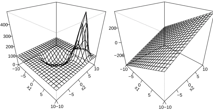
the linear kernel. Please note that such small values ofλwill result in relatively large bounds. Figure 1 shows the sensitivity curves of ˆf+ˆb := fˆn,λ+ˆbn,λ, if we add a single point z= (x,y)to the original data set, where x1=6, x2=6, and y= +1. The additional data point has a local and
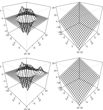
smooth impact on ˆf+ˆb with a peak in a neighborhood of(x1,x2), if one uses the RBF kernel. For a linear kernel, the impact is approximately linear. The reason for this different behavior of the SVM with different kernels becomes clear from Figure 2 where plots of ˆf+ˆb are given for the original
data set and for the modified data set, which contains the additional data point z. Please note that the RBF kernel yields ˆf+ˆb approximately equal to zero outside a central region, as almost all data
points are lying inside the central region. Comparing the plots of ˆf+ˆb based on the RBF kernel
for the modified data set with the corresponding plot for the original data set, it is obvious that the additional smooth peak is due to the new data point located at x= (6,6)with y= +1. It is interesting to note that although the estimated functions ˆf+ˆb for the original data set and for the modified data set based on the SVM with the linear kernel are looking quite similar, the sensitivity curve is similar to an affine hyperplane which is affected by the value of z. This allows the interpretation, that just a single data point can have an impact on ˆf+ˆb estimated by a SVM with a linear kernel over a broader region than for an SVM with an RBF kernel.
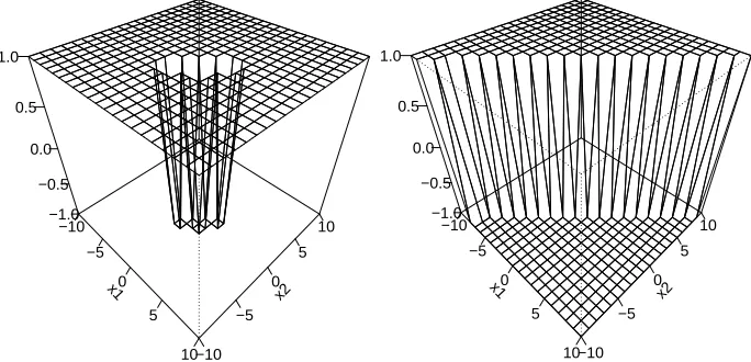
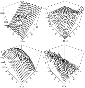
Now, we study the impact of an additional data point z= (x,y), where y= +1, on the percent of classification errors and on the fitted y−value for z. We vary z over a grid in the x−coordinates. Figure 3 shows that the percentage of classification errors is approximately constant outside the central region that contains almost all data points if a Gaussian RBF kernel was used. For the SVM with a linear kernel, the percentage of classification errors tends to be approximately constant in one half-space but changes in the other half-space. The response of the additional data point was correctly estimated by ˆy= +1 outside the central region, if a RBF kernel is used, see Figure 4. In contrast to that, using a linear kernel results in estimated responses ˆy= +1 or ˆy=−1 of the additional data point depending on the affine half-space in which the x−value of z is lying. Finally, let us study the impact of an additional data point located at z= (x,y), where y= +1, on the estimated parameters ˆb and ˆθ, see Figure 5. We vary z over a grid in the x−coordinates in the same manner as before. As the plots for ˆθ1and ˆθ2are looking very similar, we only show the latter. Note
x1
−10
−5
0
5
10
x2
−10 −5
0 5
10 0
100 200 300 400
x1
−10
−5
0
5
10
x2
−10 −5
0 5
10 −200
0 200
Figure 1: Sensitivity function of ˆf+ˆb, if the additional data point z is located at z= (x,y), where
x= (6,6)and y= +1. Left: RBF kernel. Right: linear kernel.
regions with higher sensitivity values and regions with lower sensitivity values. The sensitivity curves for the slopes of the SVM with a linear kernel are flat in one affine half-space, but change approximately linearly in the other affine half-space. This behavior also occurs for the sensitivity curve of the offset by using a linear kernel. In contrast to that, the sensitivity curve of the offset based on a SVM with a RBF kernel shows a smooth but curved shape outside the region containing the majority of the data points.
7. Concluding Remarks
In this paper, we used the influence function approach of robust statistics (Hampel et al., 1986) for recent statistical learning methods based on convex risk minimization methods for the problem of pattern recognition. The influence function has the interpretation that it measures the impact of an infinitesimal amount of contamination of the original distributionPin direction of a Dirac distribu-tion located in the point z on the theoretical quantity of interest T(P). Special cases of such convex risk minimization methods are the support vector machine, kernel logistic regression, AdaBoost, and least squares. Assumptions were derived for the existence of the influence function of f or
x1 −10 −5 0 5 10 x2 −10 −5 0 5 10 −2 −1 0 1 x1 −10 −5 0 5 10 x2 −10 −5 0 5 10 −20 −10 0 10 20 x1 −10 −5 0 5 10 x2 −10 −5 0 5 10 −2 −1 0 1 x1 −10 −5 0 5 10 x2 −10 −5 0 5 10 −20 −10 0 10 20
Figure 2: Plot of ˆf+ˆb. Upper left: RBF kernel, original data set. Upper right: linear kernel,
original data set. Lower left: RFB kernel, modified data set. Lower right: linear kernel, modified data set. The modified data set contains the additional data point z= (x,y), where x= (6,6)and y= +1.
the sensitivity curve, which can be interpreted as a finite sample version of the influence function, of the SVM classifier. It turned out, that the popular exponential radial basis function kernel resulted in smooth sensitivity curves for ˆf+ˆb and for the estimated coefficients(θˆ,ˆb). Varying the position of one additional data point had a smooth and local impact on ˆf+ˆb, if one uses an RBF kernel. For
the linear kernel the impact of varying one additional data point behaves also in a relatively smooth manner, but the impact seems to be more globally than locally.
x1 −10 −5 0 5 10 x2 −10 −5 0 5 10 28.0 28.5 29.0 x1 −10 −5 0 5 10 x2 −10 −5 0 5 10 29.2 29.4 29.6 29.8 30.0 30.2
Figure 3: Percent of classification errors if one data point z= (x,1)is added to the original data set, where x varies over the grid. Left: RBF kernel. Right: linear kernel.
x1 −10 −5 0 5 10 x2 −10 −5 0 5 10 −1.0 −0.5 0.0 0.5 1.0 x1 −10 −5 0 5 10 x2 −10 −5 0 5 10 −1.0 −0.5 0.0 0.5 1.0
Figure 4: Fitted y−value for new observation if one data point z= (x,1)is added to the original data set, where x varies over the grid. Left: RBF kernel. Right: linear kernel.
It would be interesting to study the influence function of convex risk minimization methods for other problems, e.g. ε−regression or kernel principal component analysis, or to consider other robustness concepts, but this is beyond the scope of this paper.
Acknowledgments
x1
−10
−5
0
5
10
x2
−10 −5
0 5
10 −4000
−2000 0 2000
x1
−10 −5
0
5
10
x2
−10 −5
0 5
10 −60
−40 −20 0 20
x1
−10 −5 0 5 10
x2
−10 −5
0 5
10 −10000
−5000 0
x1
−10 −5 0 5
10
x2
−10 −5
0 5
10 0
5 10
Figure 5: Sensitivity function for ˆθand ˆb, respectively. Upper left: Sensitivity function for ˆθ2, RBF
kernel. Upper right: Sensitivity function for ˆθ2, linear kernel. Lower left: Sensitivity
function for ˆb, RBF kernel. Lower right: Sensitivity function for ˆb, linear kernel.
simulation”) are gratefully acknowledged. We thank three anonymous referees and the editor for helpful remarks on an earlier version of the paper.
Appendix A. Mathematical Background
In Appendix A we list some facts from functional analysis, which are used in Appendix B to prove our theorems.
functionϕ: E→F with ϕk(xxk)→0 for x→0 such that
G(x0+x)−G(x0) = Ax+ϕ(x) (16)
for all x∈E. It turns out that A is uniquely determined by (16). As in Section 4 we hence write G0(x):= ∂G∂E(x):=A. Again, the map G is called continuously differentiable if the map x7→G0(x)
exists on E and is continuous. Analogously we define continuous differentiability on open subsets of E.
Unlike 1-dimensional derivates general Fr´echet derivates suffer from some notational difficulties. For example, the derivate G0(x)itself is a map for every x and thus G0(x)is described by y7→G0(x)y.
Furthermore, considering partial derivates can cause notational problems too. Indeed, if e.g. idE is the identity of E we have
x = id0(x)x = ∂id ∂E(x)x =
∂id(x) ∂x x
where the right expression uses standard notation. We feel that the latter can cause problems for the unexperienced reader.
As in the finite dimensional case the differential operator satisfies basic calculus, that is linearity and a chain rule
G2◦G1
0
(x) = G02(G1(x))◦G01(x)
for G1: E1→E2, G2: E2→E3whenever all derivates exist in the above equation. Furthermore, for
a bounded linear map A : E→F we have A0(x) =A for all x∈E. If G(f):=kfk2Hfor all elements
f of a Hilbert space H we find G0=2idH, where idHdenotes the identity on H.
Let us consider an example that helps to understand the differentiation steps in the following proofs. To this end letPbe a probability measure on a subset X⊂Rdand H be a RKHS of bounded continuous functions over X with feature mapΦ: X→H, i.e.Φ(x):=k(x, .), where k is the kernel of H. We consider the map G : H→Rwhich is defined by G f :=EPL◦f for all f ∈H and a twice
continuously differentiable function L :R→R. In order to compute the derivate of this map we decompose G into G=B◦A◦I, where I : H→Cb(X)is the canonical embbeding w7→ hw,Φ(.)i of H into the space of all bounded continuous functions Cb(X), A : Cb(X)→Cb(X)is defined by
f 7→L◦f and B : Cb(X)→Ris the functional f7→EPf . For the chain rule we need to compute the derivatives of these factors. Since I is linear we have I0(v)w=Iw for all v,w∈H. Analogously, the
linearity of B gives B0(f)g=EPg for all f,g∈Cb(X). As shown in the book of Akerkar (1999), we also have A0(f)g=g·(L0◦f)for all f,g∈Cb(X), i.e. A0is the multiplication operator with respect to L0◦f . Applying the chain rule to A◦I we hence find
(A◦I)0(v)w = (A0(I(v))◦I0(v))w = L0◦(Iv)·(Iw)
for all v,w∈H. As we see the brackets play an important role for the mechanic evaluation of these
derivatives. Another application of the chain rule gives
G0(v)w = B0(A◦I(v))◦(A◦I)0(v)
w = B0(A◦I(v)) (A◦I)0(v)w = EP(A◦I)0(v)w
= EPL0◦(Iv)·(Iw)
our situation we can directly compute this representation: for v,w∈H we have hEPL0◦(Iv)Φ,wi = EPL0◦(Iv)hIv,wi = EPL0◦(Iv)·(Iw),
i.e.EPL0◦(Iv)Φis a representation of G0(v). Note thatEPL0◦(Iv)Φis a H-valued Bochner-integral. For finite dimensional spacesRn theRn-valued Bochner-integral can be computed by the integrals of the n components. In general Banach spaces some problems can occur by different notions of measurability. Since in our case H is separable by the continuity ofΦ and all our functions are continuous we do not have these difficulties. In fact for compact X our Bochner-integrals can be even computed using a simple Riemann approach. For more information about Bochner-integrals we refer to Diestel and Uhl (1977) or Yosida (1974).
Since in our proofs we also have to compute the second derivate of maps of the form of G, let us now treat G00. For convenience we use the Fr´echet-Riesz representation of G0. Analogously to the above considerations we decompose G0. To this end B : Cb(X)→H denotes the operator defined by B f :=EPfΦfor all f ∈Cb(X). Furthermore, A : Cb(X)→Cb(X)is the operator A f :=
L0◦f , f ∈Cb(X). Using the Fr´echet-Riesz representation of G0 we then find G0=B◦A◦I. Now observe that B is linear. Therefore we have B0(f)g=EPgΦ for all g∈Cb(X). Moreover, we find
(A◦I)0(v)w=L00◦(Iv)Iw for all v,w∈H as above. Using the chain rule this gives
G00(v)w = B00(A◦I(v)) (A◦I)0(v)w = EP(A◦I)0(v)wΦ = EPL00◦(Iv)IwΦ
for all v,w∈H.
Our proofs also heavily rely on the implicit function theorem in Banach spaces. Therefore, we recall a simplified version of this theorem (Akerkar, 1999; Zeidler, 1986). Here and throughout this appendix BE denotes the open unit ball of a Banach space E.
Theorem 19 (Implicit function theorem) Let E,F be Banach spaces and G : E×F →F be a continuously differentiable map. Suppose that we have (x0,y0)∈E×F such that G(x0,y0) =0
and ∂G∂F(x0,y0) is invertible. Then there exists a δ>0 and a continuously differentiable map f : x0+δBE →y0+δBF such that for all x∈x0+δBE, y∈y0+δBF we have
G(x,y) =0 if and only if y= f(x).
Moreover, the derivative of f is given by
f0(x) =−
∂
G
∂F x,f(x)
−1∂
G
∂E x,f(x)
.
For the application of the implicit function theorem we have to show that certain operators are invertible. For this the following theorem which is known as the Fredholm Alternative, (Cheney, 2001) turns out to be very helpful:
Theorem 20 (Fredholm Alternative) Let E be a Banach space and S : E→E be a compact oper-ator. Then idE+S is surjective if and only if it is injective.
We also need the Krein-Milman theorem, see Yosida (1974, p. 363) or Brown and Pearcy (1977, p. 309).
Appendix B. Proofs of the Theorems
In this appendix we prove the theorems from Section 4 and Section 5. We sometimes write L(f)
instead of L(y,f(x))and L(f+b)instead of L(y,f(x) +b)to shorten the notation, if misunderstand-ings are unlikely. We use this kind of notation also for derivatives of L.
PROOF OF THEOREM 4. Let us first check that the solution fP,λ exists in our situation.
Indeed, in the proof of the existence statement by Steinwart (2002a) the compactness of X is only used to ensure K :=kI : H→`∞(X)k<∞, where`∞(X)denotes the space of all bounded functions
f : X →Requipped with the supremum norm and I is the canonical embbeding. The finiteness of this norm, however, characterizes bounded kernels. Therefore, the existence statement by Steinwart (2002a) is true in our case too.
Now, letΦ: X →H be the feature map of H as in the above example. Our analysis heavily rely
on the map G :R×H→H that is defined by
G(ε,f):=2λf+E(1−ε)P+ε∆zL
0(Y,f(X))Φ(X).
Note that for ε6∈[0,1]the H-valued expectation is with respect to a signed measure. For these measures we refer to Dudley (2002). Now as in the above example, forε∈[0,1]we obtain
G(ε,f) = ∂R
reg
L,(1−ε)P+ε∆z,λ
∂H (f). (17)
Since f7→RregL,(1−ε)P+ε∆
z,λ(f)is convex for allε∈[0,1]Equation (17) shows that we have G(ε,f) =0 if and only if f = f(1−ε)P+ε∆z,λ for such ε. Our aim is to show the existence of a differentiable functionε7→ fε defined on a small interval[−δ,δ]for someδ>0 that satisfies G(ε,fε) =0 for all ε∈[−δ,δ]. Once we have shown the existence of this function we immediately obtain
IF(z; T,P) = ∂fε ∂ε(0).
For the existence ofε7→ fεwe only have to check by Theorem 19 that G is continuously differen-tiable and that ∂G∂H(0,fP,λ)is invertible. Let us start with the first: an easy computation shows
∂G
∂ε(ε,f) =−EPL0(Y,f(X))Φ(X) +E∆zL0(Y,f(X))Φ(X). (18)
Moreover, as in the above example we find
∂G
∂H(ε,f) =2λidH+E(1−ε)P+ε∆zL00(Y,f(X))hΦ(X), .iΦ(X). (19) Since H has a bounded kernel it is a simple routine to check that both partial derivatives are continu-ous. This together with the continuity of G ensures that G is continuously differentiable, cf. Akerkar (1999).
In order to show that ∂G∂H(0,fP,λ) is invertible it suffices to show by the Fredholm Alternative that
∂G
∂H(0,fP,λ)is injective and that
defines a compact operator on H. To show the compactness we have to recall some measure theory, see Dudley (2002). Since X is assumed to be open or closed, it is a Polish space. Furthermore, Borel probability measures on Polish spaces are regular by Ulam’s theorem, i.e. they can be approximated from inside by compact sets, cf. Bauer (1990, p. 180). In our situation, this means that for all
n≥1 there exists a compact subset Xn⊂X withPX(Xn)≥1−1/n, wherePX denotes the marginal distribution ofPwith respect to X . We define a sequence of operators An: H→H by
Ang := Z
Xn×Y
L00(y,fP,λ(x))g(x)Φ(x)dP(x,y)
for all g∈H. Let us now show that all Anare compact. By the definition of Anthere exists a constant
c>0 depending onλ, L00and K such that for all g∈BH we have
Ang∈c·acoΦ(Xn), (20)
where acoΦ(Xn)denotes the absolute convex hull ofΦ(Xn). Indeed, for discrete probability mea-suresPrelation (20) follows directly from the definition using the factkgk∞≤K for g∈BH. To see the general case recall that by Krein-Milman’s theorem the set of discrete probability measures is weak∗-dense in the set of probability measures. Then (20) follows since H has the approximation property (Lindenstrauss and Tzafriri, 1977). Furthermore, sinceΦis continuousΦ(Xn)is compact and hence so is acoΦ(Xn). This shows that An is compact. In order to see that A is compact, it therefore suffices to showkAn−Ak →0 for n→∞. The latter convergence can be easily checked usingPX(Xn)≥1−1/n.
It remains to prove that A is injective. To this end for g6=0 we find
(2λidH+A)g,(2λidH+A)g = 4λ2hg,gi+4λhg,Agi+hAg,Agi
> 4λhg,Agi = 4λ
g,EPL00(Y,fP,λ(X))g(X)Φ(X)
= 4λEPL00(Y,fP,λ(X))g2(X) ≥ 0
Here, the last equation is due to the fact that BEPh=EPBh for all E-valued functions h and all
bounded linear operators B : E →F between Banach spaces E and F. A much stronger result is
given in Diestel and Uhl (1977, p. 47). The last inequality is true since the second derivative of a convex function is always nonnegative. Obviously, the above estimate shows that ∂H∂G(0,fP,λ) =
2λidH+A is injective.
We use IF(z; T,P) = ∂f∂εε(0) to derive a formula for the influence function, whereε7→ fε is the function implicitly defined by G(ε,f) =0. The implicit function theorem hence gives
IF(z; T,P) =−S−1◦∂G
∂ε(0,fP,λ), (21)
where S := ∂G∂H(0,fP,λ).
PROOF OFTHEOREM 6. Since every compact subset ofRd is closed and continuous kernels on
PROOF OF THEOREM 8. The proof is similar to that of Theorem 4. However, due to the extra variable b we have to adapt our approach. As in the proof of Theorem 4 we first point out that the solutions(fP,λ,bP,λ)∈H×Rexist. Again, this can be seen by a slight modification of the argument used by Steinwart (2002a). Now, let us define the map G :R×H×R→H×Rby
G(ε,f,b):=2λf+E(1−ε)P+ε∆zL0(f+b)Φ,E(1−ε)P+ε∆zL0(f+b)
.
Again, forε∈[0,1]the definition of G ensures
G(ε,f,b) = ∂R
reg
L,(1−ε)P+ε∆z,λ
∂(H×R) (f),
if we apply the Fr´echet-Riesz identification(H×R)0=H×R. Since Rreg
L,(1−ε)P+ε∆z,λis convex for all
ε∈[0,1]we have G(ε,f,b) =0 if and only if(f,b)minimizes RregL,(1−ε)P+ε∆
z,λfor suchε. Our aim is to apply the implicit function theorem in the way we did it in the proof of Theorem 4. However, this time the implicit function theorem will also ensure the uniqueness of the solution of (7). Obviously, this is necessary for the existence of the influence function. In order to apply Theorem 19 we need the partial derivatives of G. By an easy computation we find
∂G
∂ε(ε,f,b) =−EPL0(f+b)Φ(X) +E∆zL0(f+b)Φ(X) and
∂G
∂(H×R)(ε,f,b) =
2λidH+EεL00(f+b)hΦ, .iΦ EεL00(f+b)Φ
EεL00(f+b)Φ EεL00(f+b)
,
where we use the abbreviationEε:=E(1−ε)P+ε∆z. A routine check shows that both G and the partial derivatives are continuous and hence G is continuously differentiable.
Now, let us fix a solution(fP,λ,bP,λ)of (7). In order to show that the operator ∂(H∂G×R)(0, fP,λ,bP,λ)
is invertible it suffices to show by the Fredholm Alternative that it is injective and that
A :=
EPL00(fP,λ+bP,λ)hΦ, .iΦ EPL00(fP,λ+bP,λ)Φ
EPL00(fP,λ+bP,λ)Φ EPL00(fP,λ+bP,λ)−2λ
is a compact operator on H×R. The latter can be seen using the argument of the proof of Theorem 4. For the former let us suppose that we have an element(g,t)∈H×Rwith(2λidH×R+A)(g,t) =0. This is equivalent to the following linear system of equations
2λg+EPL00(fP,λ+bP,λ)gΦ+tEPL00(fP,λ+bP,λ)Φ = 0 (22)
EPL00(fP,λ+bP,λ)g+tEPL00(fP,λ+bP,λ) = 0. (23)
Let us first assume that t=0. Then the above system yields
2λg+EPL00(fP,λ+bP,λ)gΦ=0.
Using the techniques of the proof of Theorem 4 we easily find that this implies g=0. Therefore, we may assume without loss of generality that t=1. In order to avoid long notations we introduce the measure dµ :=L00(fP,λ+bP,λ)dP. Note that L00>0 implies µ6=0. Now, (23) yields
![Table 1: Loss functions, where v = yf(x) or v = y[ f(x)+b], respectively.](https://thumb-us.123doks.com/thumbv2/123dok_us/9842151.1970604/5.612.96.452.88.211/table-loss-functions-v-yf-x-v-respectively.webp)