Unequal Lot Sizes for Repetitive Cycle Scheduling

(1)

ISSN: 2306-9007 Moodie & Swanson (2014) 1468

I

www.irmbrjournal.com September 2014

I

nternational

R

eview of

M

anagement and

B

usiness

R

esearch

Vol. 3 Issue.3

R

M

B

R

Unequal Lot Sizes for Repetitive Cycle Scheduling

DOUGLAS R. MOODIE

Management & Entrepreneurship Department, 0404,

Coles College of Business, Kennesaw State University, 1000 Chastain Road, Kennesaw, GA 30144-5591, USA.

Email: [email protected] Tel: 470 578 3333

LLOYD A. SWANSON

Department of Quantitative Methods, Syracuse University, Syracuse, NY 13244-2130

Abstract

This paper examines the joint lot sizing problem for minimizing inventory costs for several products of constant demand made on one machine with zero cost setups but with setup times. If total demand requirements do not exceed available capacity then there is always a feasible schedule for any cycle sequence using different lot sizes. The paper describes a four-stage solution procedure, which builds upon the concept of not having any idle time or carryover inventory. The paper demonstrates that, quite often, unequal lot sizes can reduce inventory costs over equal lot sizes in the zero inventory case.

Key Words: Lot-Sizing, Scheduling, Setup Time.

Introduction

Researchers have been examining, for a number of years, the multi-product lot sizing and scheduling problem for a workstation with level demands, which Maxwell (1961) first formulated. Early efforts viewed this problem as how to make many products on one resource, one product at a time, with level known demands, linear holding costs, positive setup times, and costs independent of previous product produced. This approach ignored any raw material holding costs. The primary goal was, first, to determine lot sizes that would meet overall demand over time and, second, to develop a feasible cycle schedule using these lot sizes that would meet all demands without any backordering. The secondary objective was to minimize the setup costs and total inventory holding for finished goods amongst all feasible cycles.

This approach is quite straightforward with a common cycle production process, where there is a simple cycle of all products produced once each cycle. The advantage of such an approach is that it assures feasibility if there is enough available capacity for total production and setup times. If capacity is insufficient, it is a simple matter to increase the size of the lots and thereby reduce the proportion of time spent on setups. The reverse of this is reducing the size of lots until they just meet demand with full capacity and no idle periods. However, smaller lot sizes, and thus lower inventory holding costs, involve more setups and thus higher setup costs.

(2)

I

nternational

R

eview of

M

anagement and

B

usiness

R

esearch

Vol. 3 Issue.3

R

M

B

R

with constrained capacity. Researchers have published numerous schemes for swapping products from one part of the mini-cycle to another to solve this problem. Unfortunately, these schemes usually assume that lot sizes must be constant from one mini-cycle to another because of the quadratic nature of the combined inventory and setup cost structure. That is they assume that costs would probably increase for unequal lot sizes.

All these problems arise because of the assumption that setup costs exist. However, it is rational to assume in many cases that the firm will pay its labor regardless of whether they are producing products, performing setups, or are idle and that there are no specific setup costs such as cleaning fluids and scrap. So, instead of assuming that each setup requires both a cost and a time, this paper assumes that there are no variable costs to setups, as Pinto and Mabert (1986) or Kim, Mabert, and Pinto (1993) did.

This assumption often occurs in real life, where there are no additional, short-term costs to doing a setup over production, or such a cost is far less than inventory costs. A typical example is an aerosol filling line that fill both wax and scent aerosols with widely differing fill rates. The main variable cost of production and thus inventory costs are the costs of aerosols. Setup mainly consists of removing the previous liquid from the filling lines, which takes a period of time. This setup time varies from lengthy for cleaning wax from the lines to a short period for clearing scent from the lines. As line operators carry out the setups, there are no additional varying setup costs. In addition, when one makes the same product all the time, there is a ramp-up effect. In lines with ramp-up effects, one can account for this by using a longer setup time for the lower initial output cycles. Another example is a four-wheel drive transfer gearbox assembly line, where the line operators do the setup. As they assemble the same products all the time with level demands, there is no ramp-up effect. There is a setup time but not a setup cost.

As a result, the nature of the problem has changed, leaving inventory holding costs as the only variable cost. Now, the cost structure has changed from quadratic to linear. Also, the notion of constant lot sizes as preferable no longer holds sway. So, solutions can use unequal lot sizes for the same product, which we will show greatly simplifies the feasibility problem.

Example of Unequal Lot Sizes

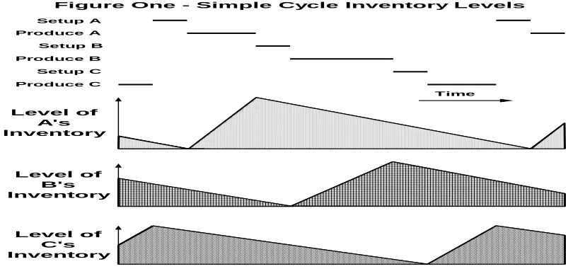
We now show pictorially how unequal lot sizes in a complex cycle can improve inventory. This example is for three products A, B, and C on one workcenter. Figure 1 shows the inventory level for each product over the life of a simple cycle. This cycle has sequence ABC and the workcenter makes each product just once a cycle.

Setup A Produce A Setup B Produce B

Produce C

Figure One - Simple Cycle Inventory Levels

Setup C

Level of A's Inventory

Level of B's Inventory

Level of C's Inventory

(3)

I

nternational

R

eview of

M

anagement and

B

usiness

R

esearch

Vol. 3 Issue.3

R

M

B

R

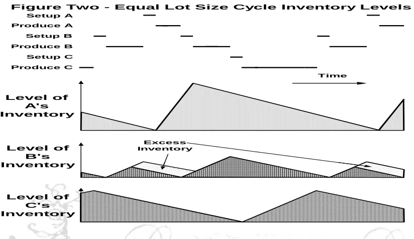
Figure 2 shows the inventory levels for products during a complex cycle (with two subcycles). This complex cycle has a sequence ABCB with equal lot sizes for B. This cycle is complex as the workcentre makes B more than once a cycle. This demonstrates that B has excess inventory as the workcentre makes A.

Setup A

Produce A

Setup B

Produce B

Produce C

Figure Two - Equal Lot Size Cycle Inventory Levels

Setup C

Excess Inventory

Time

Figure 3 shows the inventory levels for cycle ABCB with unequal lot sizes for B. Inventory profiles for A and C are the same in all three cycles. However, total inventory for B is less in Figure 3 than in the first two cycles. This shows that in this example, unequal lot sizes in a complex cycle can result in lower inventory costs than a simple cycle or equal lot sizes in a complex cycle.

Setup A Produce A Setup B Produce B Produce C

Figure Three - Unequal Lot Size Cycle Inventory Levels Setup C

(4)

I

nternational

R

eview of

M

anagement and

B

usiness

R

esearch

Vol. 3 Issue.3

R

M

B

R

Thus, the first purpose of this paper is to demonstrate how any production sequence is feasible with unequal lot sizes. After describing past research and stating the overall problem, the paper demonstrates an optimizing procedure for minimizing inventory-holding costs whilst giving feasible lot sizes for each part of a given cycle. Having demonstrated that any sequence can be feasible, the problem arises of what is the best sequence to minimize inventory costs. So, the second purpose of this paper is to show how to determine a good sequence. This involves a three-stage procedure that gives a good cycle sequence that quite often lowers inventory costs as compared to a simple cycle for a given problem. We base our procedure on the belief that good schedules should have no idle periods and each product’s inventory should run out just as production of that product resumes. We will demonstrate the simple schedule procedure with example problems. We then show solutions for these example problems using unequal lot sizes and compare them to simple schedule solutions.

Previous Work

Pinto and Mabart (1986), called henceforth P&M, developed a procedure to determine lot sizes for multi-product single workstations that uses non-repetitive sequencing for the zero cost setup case. Erenguc and Mercan (1989) criticized P&M for producing non-feasible schedules, the result of assuming equal lot sizes for each product over time. Later, Zipkin (1991) showed that constant lot sizes were not optimum for all problems with setup costs and put forward a procedure, based on Dobson’s procedure (1987) to solve the similar problem with setup costs. Allahverdi, Gupta, and Aldowaisan (1999) reviewed much of the earlier setup time literature. Sox and Gao (1999) considered setup carryover. Miller, Nemhauser, and Savelsbergh (2000), and Miller and Wolsey (2001) formulated and solved real problems with setup times and costs. Meanwhile, Ozdamar and Bozyel (2000), and Robinson and Sahin (2001) used overtime to handle the setup time problem.

Edstrom and Olhager (1987) started with the equal lot size model when investigating the value of setup time reductions. They pointed out, that for a rotating cycle with each product made each cycle, the minimum inventory holding cost comes when there is no idle time; that is, cycle time equals the sum of setup times plus the sum of production times needed for each product’s demand over the cycle time. They developed the following equation for deriving minimum cycle time,

T =



j (Sj) / [1 -



j(pj



dj)], (1)

where T is the duration of main cycle,



j is the sum for all products, Sj is the setup time, pj is the processing time, and dj is the demand rate for product j

Luss and Rosenwein (1990) used subcycles within the major cycle to schedule components made on one machine for a common assembly. They did not, though, vary their lot sizes for a given product and thus their procedure can lead to excessive inventory levels during certain periods. The research to find solutions to the joint lot sizing problem with zero setup costs has not examined using unequal lot sizes for a product in different subcycles in the production cycle.

Formulation of the Overall Problem

The Problem Restated

(5)

I

nternational

R

eview of

M

anagement and

B

usiness

R

esearch

Vol. 3 Issue.3

R

M

B

R

constant lot sizes over time. The workcentre does not need to make every product every subcycle. The firm must meet all demand with no back orders. The study assumes that sufficient inventories exist to allow the first cycle to begin. The problem is to find a feasible sequence and the corresponding lot sizes that minimize inventory costs.

Symbols Used

In order to help develop this procedure, this paper and attachments will use the following symbols throughout in its equations and writings,

A is the number of production hours in a year

AHCj is the total annual inventory holding cost for product j AIj is the average inventory for product j

Cj is the inventory holding cost for product j per cycle dj is the demand rate per hour for product j

Dj is the annual demand for product j

eij is the idle time after producing product j in subcycle i hj is the holding cost rate in $s per hour for product j Hj is the annual holding cost rate in $s for product j

Iij is total inventory for product j from subcycle i to subcycle i + yj Ij is total inventory for product j over the cycle

i is the subcycle number in the cycle j is the product number or name k is the sequence number

kij is the value of sequence number k for product j in subcycle i lij is the lot size for product j in subcycle i

m is the number of products

n is the number of subcycles in the main cycle, = max(zj) = zmax p_j is the production rate per hour for product j

ptj is the processing time in hours to make one product j

rij is the time, in hours, from the end of making product j in subcycle i, until the start of making product j again, which is not necessarily in the next subcycle.

Sj is the setup time, in hours, for product j



i means the sum for all subcycles from i = 1 to i = n



_{j means the sum for all products from j = 1 to j = m}

tij is the production time in hours for product j's lot in subcycle i T is the total time in hours of the main cycle

T_max is the maximum total time in hours of the main cycle allowed TAHC is the total annual inventory holding cost for all products xij is whether product j is made in subcycle i; xij = 1 if yes, xij = 0 if no yj is the number of subcycles until product j is next made, as defined by P&M y_{is the vector of yjs, viz., [ y1}, y₂, . . . . , y_m]

zj is the number of times in a cycle product j is made; = S xij z_{is the frequency vector of zjs, viz. , [ z1}, z₂, . . . . , z_m]

z is the infeasible optimum frequency vector [ z₁



, z₂



, ... , z_m



]

(6)

I

nternational

R

eview of

M

anagement and

B

usiness

R

esearch

Vol. 3 Issue.3

R

M

B

R

Formulation

We will first formulate the overall problem assuming no idle time using the symbols defined above. Appendix A reformulates the problem for cases with idle time. In a complex cycle there are several subcycles in each cycle. The firm makes each product every cycle but not necessarily every subcycle. A product appears at most once each subcycle. The objective function is minimizing inventory cost per time,

MIN



_{j (hj}



Ij /T) (2)

The machine makes product j for time tij in subcycle i. A time rij passes before the machine begins to make j again just as j's inventory runs out. Over this time, the total inventory is peak inventory multiplied by the period between the starts of producing j, tij + rij, divided by 2. Inventory built up during period tij dissipates during period rij. This is because any excess inventory existing when production restarts will add to the unnecessary inventory holding costs and not enough inventory will lead to stock-outs. So, the peak inventory of product j is the maximum inventory built up. In equation form, it is,

(p_j - d_j)



_{tij = d}j



rij (3)

Thus, total inventory for product j between productions is,

Iij = [tij + (pj - dj)



tij /dj]



(pj - dj)



tij/2 (4) Iij = [pj



(pj - dj)



tij2] / (2



_dj). (5) Thus for product j, the holding cost per cycle is the sum of the inventories for each buildup multiplied by the holding cost,

Cj = hj



pj



[(pj - dj)/(2



dj)]



i {tij 2

} (6)

Since the total holding cost rate for the schedule is the sum of the product holding costs divided by the cycle length, the objective function minimizes the sum of the results of average inventories multiplied by their holding cost rates. Thus, it is necessary to solve,

MIN



_{j [hj}



_pj



_{(pj - dj)/(2}



_dj)



_{i (tij}2/T)], (7) where the cycle length, T, is the sum of setup times and production periods,

T =



_{j (zj}



_{Sj +}



_{i tij)} (8)

zj =



i (xij) >= 1, integer, for all j (9) where xij is whether product j is produced in subcycle i and each product must be made at least once each cycle.

There must be a balancing of demand and production. So reformulating equation (3) gives,

tij = dj



rij / (pj - dj) for all tij (10)

where the period the inventory built up for product j in subcycle i is the total of all setups and production periods until product j is in production again in subcycle q,

k=kiq-1

rij =



k {(tij + xij



Sj), with i and j from kij} (11) k=k_ij+1

Finally, one converts production periods into lot sizes,

lij = pj



tij for all i, for all j (12)

(7)

I

nternational

R

eview of

M

anagement and

B

usiness

R

esearch

Vol. 3 Issue.3

R

M

B

R

our four-stage procedure for this step and the rationale behind it. Second, find the minimum lot sizes for this sequence that are feasible. We will later show how one can find the minimum feasible lot sizes for any given sequence.

Determining a Realistic Cycle Sequence

The fact, shown later, that a feasible schedule exists for any sequence leads to the necessity of finding the best sequence. Due to the continuous nature of the lot sizes and the discrete nature of the setup time, this can be a difficult problem. However, the following procedure offers a good solution. This procedure uses the fact that for any one product then equal lot sizes at equal spacing will always give a lower cost for that product than unequal lot sizes. However, often this would lead to more than one product being scheduled at the same time or alternately product either running out before resumption of product or else inventory not running out just as production restarts. One wants inventory to run out as production restarts or else one has stored product from one production run to the next. This creates unwanted holding costs. Thus, in many cases equal lot sizes for anything more complicated than a simple cycle are infeasible. Thus, one has to stretch what is cheapest for each product to get an overall feasible schedule that has a low cost. The next section outlines the procedure, while later sections discuss each part of this procedure in more detail.

General Procedure

The proposed procedure consists of the four stages, outlined below:

1) Find the optimum frequency vector, z. That is one decides what is the ratio of product lots in a cycle, assuming equal lot sizes for each product over a very large Tmax. As one is dealing with frequencies, this stage takes no account of the limitation that one can only make one product at a time or that one wants inventory to just run out as production restarts. It also does not produce integer number of lots per cycle.

So it can be an infeasible frequency vector. Convert this z* to a feasible but extremely long z+ by multiply

by a large factor, like 1000, until all the zj*s are integer zj+s. The cost of this z becomes the lowest cost bound.

2) Find a good frequency integer vector, z, from with a suitable T. That is one decides how many times a cycle to produce each product. The cost of this z with equal lot sizes becomes the lower bound of this frequency vector. This lower bound is normally infeasible. One should repeat the second stage if the gap between the lowest bound and the lower bound is too large. These lower bounds are quick checks to ensure one is on the right track, since the equal lot size calculations are quick although they normally produce infeasible solutions.

3) Use the determined frequency vector, z, to find a good and practical sequence. The firm can find this sequence manually using a near equal spacing procedure or with some procedure like that of Zipkin (1991).

4) Find the minimum cycle length, T, and the feasible lot sizes for that sequence when there is no idle time. Then one compares the cost with the lower bound cost for that z. One should repeat the third stage if the gap is too large.

Determining the Frequency Vector, z*

The derivation of the following equations, (12) to (16), which find z* _{for a given Tmax, is in Appendix 2} because of its length.

MIN



_{j (bj/zj}*) (13)

(8)

I

nternational

R

eview of

M

anagement and

B

usiness

R

esearch

Vol. 3 Issue.3

R

M

B

R

Such that,

zj* >= 1 , for all j (15)



j (Sj



zj*) <= Tmax



[1 -



j (dj/pj)] (16)

For the case with a common setup time, S, the constraint (16) becomes,



_{j (zj*) <= Tmax}



[1 -



_{j (dj/pj)] / S} (17)

These equations find a frequency vector, z*, which minimizes annual inventory costs for a cycle of length Tmax. These equations find the ratios of zjs while assuming that all the tij for each product j are the same. This assumption makes the problem easily solvable but usually the tijs will not be the same. The value of Tmax does not matter as long as it is large because it is only the ratio of the zj*s that matters at this stage. Then multiply z* by a constant to get z+ _{whose zj+ are all integer. One can get the cost of the feasible}

lowest bound if one assumes equal lot sizes for this z.

Determining the Frequency Vector, z

Make all the final zjintegers by manually rounding the resulting non-integer zj*s. One rounds the zj*s results in most cases for a very small cost rise, as the cost structure is relatively robust. The rounded zj*s gives the zjs that forms the trial zs. One can calculate the lower bound for any z by assuming equal lot sizes. This is because unequal lot sizes for any z will cost more than equal but unfeasible lot sizes. The upper bound cost is the cost of a simple sequence. The optimal feasible solution must be worse than the lowest bound. A good z is as a result defined as a z whose lower bound cost is less than that of the simple cycle solution cost and that is not too much above the lowest bound cost.

Determining sequence from frequency vector, z

The best sequence would minimize the inventory holding costs such that products just run out of inventory as production restarts. Thus, to find lot sizes, solve the following equations,

MIN



_{j [cj}





_{i (tij}2)] such that (10), (11), and (12) are true, (18)

where cj = Hj



pj



(pj - dj) / dj (19)

There are several different possible sequences for each z. To compare the possible sequences, it is necessary to compute for each sequence, the feasible lot sizes and the resultant inventory holding cost. We suggest that one chooses a sequence manually by trying to space product runs such that the period between production restarts, rij’s, for each j are near to the same as possible. One does this by scheduling the products with the highest cjs with as near to equal lot sizes as possible, then fitting in the others. This method is works well for small zs and a small number of products. Zipkin’s (1991) procedure for a multi-product case would also work for this case if one lets his u and an equal zero. Pair-wise exchange techniques can also produce variation on an initial sequence. We found that our examples had little cost variations with different sensible sequences for the same z. Appendix 2 determines the lower bound cost,

which is T



_{j (bj/zj) / 2.} (20)

Development of the Cycle Length Equation

(9)

I

nternational

R

eview of

M

anagement and

B

usiness

R

esearch

Vol. 3 Issue.3

R

M

B

R

larger lot sizes and thus inventory costs and a smaller length will lead to stock outs. With this cycle length there is no idle time. So, one calculates the total cycle setup time for the given cycle sequence. The annual available time for setups is the available capacity minus the total processing time for the total annual demand of all products. One obtains the number of cycles per year (N) by dividing the total annual setup time available by the required cycle setup time. The cycle’s total length, T, is the annual available capacity, A, divided by the number of cycles,

T = A/N =



_{j {(Sj}



_zj)



A / [A -



_{j (Dj/pj)]}} (21)

Determining the lowest cost feasible lot sizes for a cycle sequence

Use the equations (8), (10), (11), and (12) to produce the minimum lot sizes for the chosen sequence. One repeats this for several sequences derived from z and chooses the lowest cost sequence. We demonstrate this procedure with the following sample problems.

Examples

Sample Problems

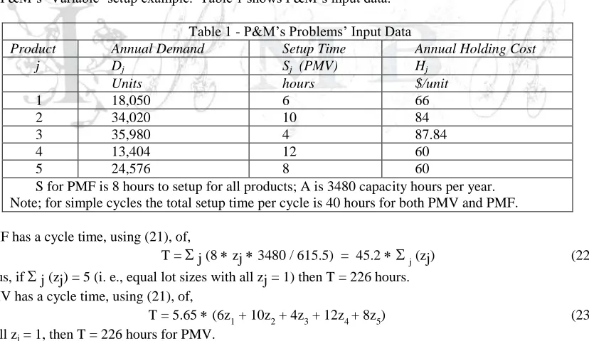
We will use P&M’s two example problems’ input data to show how to use these equations for actual problems. P&M’s first example problem has equal setups with different holding and demand rates for each of the five products. We shall call this PMF for P&M’s ‘Fixed’ setup example. P&M’s second example has unequal setup times but has all other numbers the same as problem PMF. We call this problem PMV for P&M’s ‘Variable’ setup example. Table 1 shows P&M’s input data.

Table 1 - P&M’s Problems’ Input Data

Product Annual Demand Setup Time Annual Holding Cost

j Dj Sj (PMV) Hj

Units hours $/unit

1 18,050 6 66

2 34,020 10 84

3 35,980 4 87.84

4 13,404 12 60

5 24,576 8 60

S for PMF is 8 hours to setup for all products; A is 3480 capacity hours per year. Note; for simple cycles the total setup time per cycle is 40 hours for both PMV and PMF.

PMF has a cycle time, using (21), of,

T =



_{j (8}



_zj



3480 / 615.5) = 45.2



_{j (zj)} ₍₂₂₎

Thus, if



_{j (zj) = 5 (i. e., equal lot sizes with all zj = 1) then T = 226 hours.} PMV has a cycle time, using (21), of,

T = 5.65



(6z_{1 + 10z2 + 4z3 + 12z4}+ 8z₅) (23) If all zj = 1, then T = 226 hours for PMV.

Fixed Lot Schedule

(10)

I

nternational

R

eview of

M

anagement and

B

usiness

R

esearch

Vol. 3 Issue.3

R

M

B

R

lj = dj



T for all j (24)

For a simple cycle, as average inventory is half the maximum inventory and maximum inventory is lj



(pj - dj)/pj, then product annual holding cost is from,

AHCj = Hj



lj



(pj - dj) / (2



pj) (25)

For these particular problems, PMF and PMV, since the lot sizes are identical, the constant lot size solution gives a feasible schedule with a annual inventory cost of $249,016. This is the cost that we will use as an upper bound for future comparisons.

Unequal lot schedule results for P&M's examples

This procedure gives feasible solutions with unequal lot sizes to the two P&M problems. We solved, by

giving non-integer zj*s, these nonlinear equations for optimality for a Tmax of half a year. We rounded the resulting zj*s to give feasible z_{s with integer zjs. We then choose sequences for each problem, calculated} lot sizes, and thus annual inventory costs for these sequences.

Results for example PMF

The solution for the PMF example is a non-integer answer z+,

z+ = [6.62, 9.63, 10.04, 5.53, 7.18]

We converted this z+ into a good but not very practicable integer z*, _{by multiplying zj+ by 100, which} keeps the same ratio of production lots per cycle,

z* = [662, 963, 1004, 553, 718]

This z* would require 3900 setups per cycle and take 50.7 years.

We thus converted the original infeasible z+ to the following four feasible zs, which are more practical than

z*_{, by rounding the original zj*s. The total number of subcycles in a cycle is made equal to the largest zj.} We first chose a z with five subcycles then further rounded to get one with four subcycles. This rounding continued until we had a z of two subcycles. We manually chose for each z the following associated sequences that keep a particular product’s spacing as constant as possible. This is because for any particular product and cycle length equal spacing minimizes holding costs. These sequences may not be the optimum sequences for these particular zs. We also worked out a sequence for P&M’s original solution for comparison.

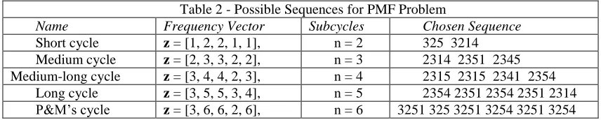
P&M had for the PMF problem, after their rounding, a subcycle interval vector of y_{= [2, 1, 1, 3, 1]. zmax} is the smallest integer from P&M's y_{of which all yj are integer factors. This gives a zmax of 6. We} converted y to a frequency vector, z_{= [3, 6, 6, 2, 6], by using zj = zmax/yj. We selected possible} sequences based on this frequency vector, which are listed in Table 2.

Table 2 - Possible Sequences for PMF Problem

Name Frequency Vector Subcycles Chosen Sequence

Short cycle z = [1, 2, 2, 1, 1], n = 2 325 3214 Medium cycle z = [2, 3, 3, 2, 2], n = 3 2314 2351 2345 Medium-long cycle z = [3, 4, 4, 2, 3], n = 4 2315 2315 2341 2354

(11)

I

nternational

R

eview of

M

anagement and

B

usiness

R

esearch

Vol. 3 Issue.3

R

M

B

R

For each z, we found the lower bound using equation (20). For each sequence, we found the cycle length and average inventory holding rate using equations (7), (8), (10), (11), and (12). Annual holding cost is inventory holding rate multiplied by the annual capacity. Table 3 shows the results, which Figure 4 graphically presents.

Table 3 - Summary of results for PMF problem

Subcycles T Annual Inventory Cost ($)

n hours Lower Bound Actual Comments

1 226 249,016 249,016 Upper bound

2 317 243,061 243,879 Best actual

3 543 238,548 244,036

4 724 238,172 250,049

5 905 238,168 255,180 Best lower bound

6 1041 n.a. 263,653 P&M’s solution

1004 176,338 237,090 237,090 Lowest bound

Comments on PMF’s results

The lower bound did become lower with more subcycles but the improvement rapidly became small. The lowest bound gave a 4.8 % improvement over a simple cycle. However, the lowest bound is not feasible. Thus, one must use one of the feasible, non-optimal sequences. Interestingly, the gap between the actual cost and the lower bound cost increased as the number of subcycles increased, possibly due to the discrete aspects of the problem. The lowest actual cost found was for a sequence of two subcycles, which gave a 2.1 % improvement over the simple sequence. This improvement is almost half of the maximum possible. P&M’s solution was 5.8 % worse than a simple cycle.

Results for example PMV

The solution for the PMV example is a non-integer z+,

(12)

I

nternational

R

eview of

M

anagement and

B

usiness

R

esearch

Vol. 3 Issue.3

R

M

B

R

We converted this by multiplying by 100 into a z = [784, 883, 1455, 463, 737] with an impracticable cycle time of 50 years. We produced from this z



and the three practicable and feasible zs by continually rounding.

P&M used a subcycle spacing vector y = [3, 2, 1, 7, 2] for the unequal setup time problem, PMV. We changed P&M’s y₄ to 6 from 7 for this paper as P&M had already rounded up their original y = [29, 16, 10, 69, 21]. Using their y would have resulted in 42 subcycles and a cycle time of over a year and a half, which we considered as too long. This y gave a frequency vector z = [2, 3, 6, 1, 3]. We chose manually for each z the following sequences in Table 4, where product spacing is as constant as possible.

Table 4 - Possible Sequences for PMV Problem

Name Frequency Vector Subcycles Chosen Sequence

Short cycle z = [1, 1, 2, 1, 1], n = 2 12345 3 Medium cycle z = [2, 2, 3, 1, 2], n = 3 325 312 3541 Long cycle z = [2, 2, 4, 1, 2], n = 4 134 235 13 235 P&M’s solution z = [2, 3, 6, 1, 3], n = 6 321 35 32 351 32 354

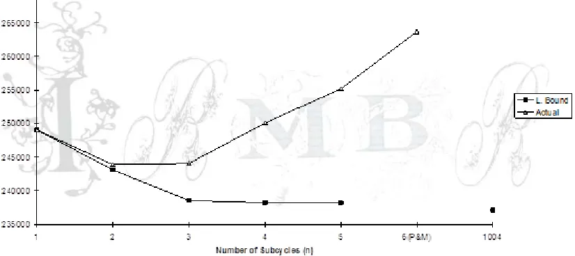
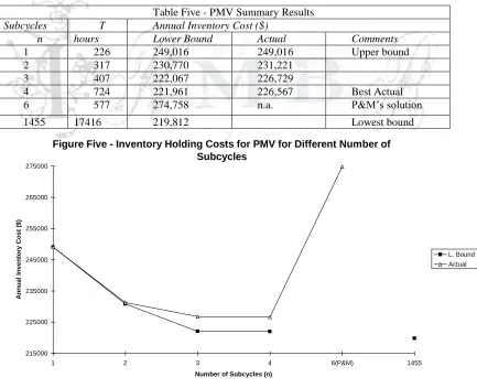
As with problem PMF, we found the lower bound for each z. For each sequence, we found the cycle length and average inventory holding rate and compared the actual and lower bound holding costs for each sequence. We tabulate the results in Table 5 and graphically present them in Figure 5.

Table Five - PMV Summary Results

Subcycles T Annual Inventory Cost ($)

n hours Lower Bound Actual Comments

1 226 249,016 249,016 Upper bound

2 317 230,770 231,221

3 407 222,067 226,729

4 724 221,961 226,567 Best Actual

6 577 274,758 n.a. P&M’s solution

1455 17416 219,812 Lowest bound

Figure Five - Inventory Holding Costs for PMV for Different Number of Subcycles

215000 225000 235000 245000 255000 265000 275000

1 2 3 4 6(P&M) 1455

Number of Subcycles (n)

A

n

u

a

l

In

v

e

n

to

ry

C

o

s

t

($

)

(13)

I

nternational

R

eview of

M

anagement and

B

usiness

R

esearch

Vol. 3 Issue.3

R

M

B

R

Comments on PMV’s Results

This example shows that an unequal lot sequence in this instance gives a saving of $22,167 over the simple cycle’s cost. The lower bound became lower with more subcycles, but the improvement rapidly became small with a lowest lower bound of an 11.7 % improvement over a simple cycle. The gap between the actual cost and the lower bound cost increased as the number of subcycles increased. The best actual lowest cost found was for a four subcycle sequence. The difference, however, between the three and four subcycle costs was minimal. This result gave a 9 % improvement over the simple sequence. This is over three-quarters of the maximum possible improvement. P&M’s feasible solution was 10.3 % worse than the simple cycle solution in this instance.

Finding lot sizes and annual holding cost

We now show the details of finding the cycle length and annual holding cost for one sequence as an example in Table 6.

Table Six - Example: Detailed Results for PMV with short cycle Cycle sequence is 12345 3

Period tij

Run Hours

pj - dj

units/hr

tij + rij

hours

Subcycle Inventory

Average Inventory

H j

($)

Annual j's InvCost

Lot Size

t13 26. 33 33. 66 112. 03 49637 1158

t23 32. 15 33. 66 136. 81 74032 496. 98 $87. 84 $43,655 1415 t12 55. 31 34. 22 248. 84 235513 946. 438 $84. 00 $79,501 2434 t11 29. 35 38. 81 248. 84 141746 569. 623 $66. 00 $37,595 1291 t15 39. 93 36. 94 248. 84 183503 737. 429 $60. 00 $44,246 1757 t14 21. 77 40. 15 248. 84 108762 437. 074 $60. 00 $26,224 958

Setups 44. 00

Total 248. 84 $231,221 9013

Conclusions

This paper demonstrates that there exists a feasible set of lot sizes for all sequences with zero setup costs. Using zero setup costs often makes more sense in many instances rather than assigning variable setup costs. The procedure nearly minimizes inventory costs in all but special instances for the zero setup cost case. One should consider unequal lot sizes to helping generate solutions in other scheduling problems as sequences with unequal lot sizes will usually give reduced inventory costs over equal lot size sequences.

A more complicated sequence, where a product is not in production every subcycle, can lessen costs. A much more complicated sequence, however, may not be worthwhile. Although the lower bound cost decreases with longer cycle times, the actual achieved costs may not decrease. This is because it is more difficult, with more complex frequency vectors to approach the lower bound schedule. It may not be worthwhile because of this, and because of the rapid tailing off of the cost improvement with extra subcycles, to look at very long cycle times. Although all the example problems had the same processing times, this procedure will work with different processing times for each product.

(14)

I

nternational

R

eview of

M

anagement and

B

usiness

R

esearch

Vol. 3 Issue.3

R

M

B

R

Similarly, one can use this procedure to value setup time reduction and to find out which product’s setup time to reduce. It is often worth reducing setup times even when not it appears the plant is not producing at full capacity. In the extreme with very small setup times, one can have lot sizes of one and thus minimal inventory costs.

Appendix 1 - Adapting the procedure for idle time or carryover inventory

Having an idle period after a small lot and before a large lot can help to lower average inventory by increasing the preceding small lot. This can reduce inventory costs for the product of that small lot if that lot was relatively small compared with other lot sizes of the same product. Lowering the average inventory for that product causes this. That maximum will hold sway over a smaller portion of a longer cycle time although the maximum inventory may remain the same or even increase. Enlarging the small lot will increase the size of all the other product lots that it overlaps. There will be further subsequent effects caused by these increasing lot sizes.

The cycle time must increase by more than the idle time inserted in the schedule. The savings, if any, from the idle time for one product will be in many cases less than the extra costs for the other products that have to have larger lot sizes. One could consolidate the idle periods to allow a setup and a new production period that will reduce inventory costs. One will in this case be changing the sequence. We consider that if one can reduce the inventory cost by using idle time then there is probably a better sequence available. So, one should not have planned idle time.

If however one wants idle times, eijs, one can still obtain a feasible schedule. Equation (11) now becomes,

rij = eij +



i



j (tij + xij



Sj) (25)

This gives (



_{zj + the number of eijs) unknowns in}



_{(zj) equations. One could use an objective function if} one wanted to minimize cycle length,

MIN T =



_i



_{j (tij + eij) +}



_{j (zj}



_Sj) (26)

The formulation includes any needed carryover inventory. Any extra carryover inventory acts as safety stock and thus does not affect the decision-making.

Appendix 2 – Derivation of a formulation to find z

One wants to minimize total inventory cost. So for product j in subcycle i,

Maximum Iij = (pj - dj)



tij (27)

Total inventory over period i from start of production of product j until we next start to make product j is maximum inventory times time between production starts divided by two,

Iij = (pj - dj)



tij



(tij + rij)/2 (28)

Total inventory for product j over the cycle of length T is the sum of all subcycle inventories,

Ij =



i [(pj - dj)



tij



(tij + rij)] /2 (29)

Average inventory for product j is total inventory divided by time T,

(15)

I

nternational

R

eview of

M

anagement and

B

usiness

R

esearch

Vol. 3 Issue.3

R

M

B

R

AHCj =



i [(pj - dj)



tij



(tij + rij)] / (2



T) (32) Total inventory holding cost is the sum of all the individual product holding costs,

TAHC =



_{j {Hj}



_{(pj - dj)}



_{i [tij}



_{(rij + tij)]} / (2}



T) (33) Now, demand during time, rij equals net production in time tij,

(pj - dj)



tij = dj



rij for all i and for all j (3) Rearranging (3),

rij = (pj/dj - 1)



tij for all i and for all j (34) Substituting (34) in (33),

TAHC =



_{j {[Hj}



_{(pj - dj)}



_pj/dj



_{i (tij}2)] / (2



T)} (35)

Total setup time per cycle =



_{j (Sj}



_zj) (36)

Total production time per cycle =



_{j (dj/pj)}



T

(37) Adding (36) and (37) gives T,

T =



_{j (Sj}



_{zj) +}



_{j (dj/pj)}



T (38)

Rearranging (38),



_{j {(Sj}



_{zj) = T}



[1 -



_{j (dj/pj)]}} (39) Thus rearranging (39),

T =



_{j {(Sj}



_{zj) / [1 -}



_{j (dj/pj)]}} (40) So problem using (33) becomes,

MIN



_{j {[Hj}



_{(pj - dj)}



_pj/dj



_{i (tij}2)] / (2



T)} (41) Such that,

T =



_{j {(Sj}



_{zj) / [1 -}



_{j (dj/pj)]}} (40)

zj >= 1 and is integer for all j (9)

Simplification

We try to find a minimum lower bound case to solve this problem. This is the minimum



_{i (tij}2), which is

when all tij for one product j are equal to tj as



i (tij) in a cycle is a constant. This is usually not a feasible solution. So, we assume tij = tj, for all j. Thus substituting,



i (tij 2

) = zj



tj2 for all j (42)

Now in each cycle,

zj



tj



pj = dj



T (production = demand for each j) (43) Rearranging (43),

tj = dj



T / ( pj



zj) (44)

Substituting (44) in (42),



i tij 2

= zj



[dj



T / (pj



zj)]2

= dj2



T2_{/ (pj}2



_zj) (45) So (41) becomes after the substitution of (45) in the objective function,

MIN (T/2)



_[Hj



_dj



_{(pj - dj) / (pj}



_zj)] (46) So the problem becomes by substituting bj (14) in objective function (46),

MIN (T/2)



_{j (bj/zj)} (47)

Such that,



j (Sj



zj) = T



[1 -



j (dj/pj)] (40)

(16)

I

nternational

R

eview of

M

anagement and

B

usiness

R

esearch

Vol. 3 Issue.3

R

M

B

R

References

Allahverdi, A., Gupta, J. N. D., and Aldowaisan, T. (1999) A review of scheduling research involving setup considerations. Omega, 27, 219-239.

Dobson, G. (1987) The economic lot sizing problem: achieving feasibility using time varying lot sizes.

Operations Research, 35, 764-771.

Edstrom, A., and Olhager, J. (1987) Production economic aspects on setup efficiency. Engineering Costs

and Production Economics, 12, 99-106.

Erenguc, S. S., and Mercan, H.M. (1989) On the joint lot sizing problem with zero setup costs. Decision Sciences, 20 (4), 669-676.

Kim, D. S., Mabert, V. A., and Pinto, P. A. (1993) Integrative cycle scheduling approach for a capacitated flexible assembly system. Decision Sciences, 24, 126-147.

Luss, H., and Rosenwein, M. B. (1990) A lot-sizing model for just-in-time manufacturing. Journal of the

Operational Research Society, 41(3), 20-09.

Maxwell, W. L. (1961) An investigation of multi-product, single-machine scheduling and inventory problems. Cornell University Ph.D. Thesis. Ithaca, NY.

Miller, A. J., Nemhauser, G. L., and Savelsbergh, M.W.P. (2000) Solving multi-item capacitated lot-sizing problems with setup times by branch-and-cut. CORE Discussion Paper 2000/39. Universite Catholique de Louvain, Belgium.

Miller, A. J., and Wolsey L. A. (2001) Tight MIP formulations for multi-item discrete lot-sizing problems.

CORE Discussion Paper 2001. Universite Catholique de Louvain, Belgium.

Ozdamar, L., and Bozyel, M. A. (2000) The capacitated lot sizing problem with overtime decisions and setup times. IIE Transactions, 32, 1043-1057.

Pinto, P. A., and Mabart, V. A. (1986) A joint lot sizing rule for fixed labor cost situations. Decision Sciences, 17 (1), 139-150.

Robinson, E.P., and Sahin, F. (2001). Economic production lot sizing with periodic costs and overtime.

Decision Sciences, 32 (5), 423- 452.

Sox, C. R., and Guo, Y. (1999) The capacitated lot sizing problem with setup carry-over. IIE Transactions,

31, 173-181.