Building Support Vector Machines with Reduced Classifier Complexity

(1)

Building Support Vector Machines with

Reduced Classifier Complexity

S. Sathiya Keerthi [email protected]

Yahoo! Research

3333 Empire Avenue, Building 4 Burbank, CA 91504, USA

Olivier Chapelle [email protected]

MPI for Biological Cybernetics 72076 T¨ubingen, Germany

Dennis DeCoste [email protected]

Yahoo! Research

3333 Empire Avenue, Building 4 Burbank, CA 91504, USA

Editors: Kristin P. Bennett and Emilio Parrado-Hern´andez

Abstract

Support vector machines (SVMs), though accurate, are not preferred in applications requiring great classification speed, due to the number of support vectors being large. To overcome this problem we devise a primal method with the following properties: (1) it decouples the idea of basis functions from the concept of support vectors; (2) it greedily finds a set of kernel basis functions of a specified maximum size (dmax) to approximate the SVM primal cost function well; (3) it is

efficient and roughly scales as O(nd2

max)where n is the number of training examples; and, (4) the

number of basis functions it requires to achieve an accuracy close to the SVM accuracy is usually far less than the number of SVM support vectors.

Keywords: SVMs, classification, sparse design

1. Introduction

Support Vector Machines (SVMs) are modern learning systems that deliver state-of-the-art perfor-mance in real world pattern recognition and data mining applications such as text categorization, hand-written character recognition, image classification and bioinformatics. Even though they yield very accurate solutions, they are not preferred in online applications where classification has to be done in great speed. This is due to the fact that a large set of basis functions is usually needed to form the SVM classifier, making it complex and expensive. In this paper we devise a method to overcome this problem. Our method incrementally finds basis functions to maximize accuracy. The process of adding new basis functions can be stopped when the classifier has reached some limiting level of complexity. In many cases, our method efficiently forms classifiers which have an order of magnitude smaller number of basis functions compared to the full SVM, while achieving nearly the same level of accuracy.

(2)

of solving the following primal problem

minλ 2kwk

2₊1 2

n

∑

i=1

max(0,1−yiw·φ(xi))2. (1)

Computations involvingφare handled using the kernel function, k(xi,xj) =φ(xi)·φ(xj). For conve-nience the bias term has not been included, but the analysis presented in this paper can be extended in a straightforward way to include it. The quadratic penalization of the errors makes the primal objective function continuously differentiable. This is a great advantage and becomes necessary for developing a primal algorithm, as we will see below.

The standard way to train an SVM is to introduce Lagrange multipliersαi and optimize them by solving a dual problem. The classifier function for a new input x is then given by the sign of ∑iαiyik(x,xi). Because there is a flat part in the loss function, the vectorαis usually sparse. The xi for whichαi6=0 are called support vectors (SVs). Let nSV denote the number of SVs for a given

problem. A recent theoretical result by Steinwart (Steinwart, 2004) shows that n_SV grows as a linear function of n. Thus, for large problems, this number can be large and the training and testing complexities might become prohibitive since they are respectively, O(n nSV+nSV3)and O(nSV).

Several methods have been proposed for reducing the number of support vectors. Burges and Sch¨olkopf (1997) apply nonlinear optimization methods to seek sparse representations after building the SVM classifier. Along similar lines, Sch¨olkopf et al. (1999) use L1regularization onβto obtain sparse approximations. These methods are expensive since they involve the solution of hard non-convex optimization problems. They also become impractical for large problems. Downs et al. (2001) give an exact algorithm to prune the support vector set after the SVM classifier is built. Thies and Weber (2004) give special ideas for the quadratic kernel. Since these methods operate as a post-processing step, an expensive standard SVM training is still required.

Direct simplification via basis functions and primal Instead of finding the SVM solution by maximizing the dual problem, one approach is to directly minimize the primal form after invoking the representer theorem to represent w as

w=

n

∑

i=1

βiφ(xi). (2)

If we allowβi 6=0 for all i, substitute (2) in (1) and solve for theβi’s then (assuming uniqueness of solution) we will getβi =yiαi and thus we will precisely retrieve the SVM solution (Chapelle, 2005). But our aim is to obtain approximate solutions that have as few non-zero βi’s as possible. For many classification problems there exists a small subset of the basis functions1 suited to the complexity of the problem being solved, irrespective of the training size growth, that will yield pretty much the same accuracy as the SVM classifier. The evidence for this comes from the empir-ical performance of other sparse kernel classifiers: the Relevance Vector Machine (Tipping, 2001), Informative Vector Machine (Lawrence et al., 2003) are probabilistic models in a Bayesian setting; and Kernel Matching Pursuit (Vincent and Bengio, 2002) is a discriminative method that is mainly developed for the least squares loss function. These recent non-SVM works have laid the claim that they can match the accuracy of SVMs, while also bringing down considerably, the number of basis functions as well as the training cost. Work on simplifying SVM solution has not caught up well

(3)

with those works in related kernel fields. The method outlined in this paper makes a contribution to fill this gap.

We deliberately use the variable name,βiin (2) so as to interpret it as a basis weight as opposed to viewing it as yiαi whereαi is the Lagrange multiplier associated with the i-th primal slack con-straint. While the two are (usually) one and the same at exact optimality, they can be very different when we talk of sub-optimal primal solutions. There is a lot of freedom when we simply think of theβi’s as basis weights that yield a good suboptimal w for (1). First, we do not have to put any bounds on the βi. Second, we do not have to think of aβi corresponding to a particular location relative to the margin planes to have a certain value. Going even one more step further, we do not even have to restrict the basis functions to be a subset of the training set examples.

Osuna and Girosi (1998) consider such an approach. They achieve sparsity by including the L1 regularizer,λ1kβk1 in the primal objective. But they do not develop an algorithm (for solving the modified primal formulation and for choosing the rightλ1) that scales efficiently to large problems.

Wu et al. (2005) write w as

w=

l

∑

i=1

βiφ(x˜i)

where l is a chosen small number and optimize the primal objective with the βi as well as the ˜

xi as variables. But the optimization can become unwieldy if l is not small, especially since the optimization of the ˜xiis a hard non-convex problem.

In the RSVM algorithm (Lee and Mangasarian, 2001; Lin and Lin, 2003) a random subset of the training set is chosen to be the ˜xi and then only theβi are optimized.2 Because basis functions are chosen randomly, this method requires many more basis functions than needed in order to achieve a level of accuracy close to the full SVM solution; see Section 3.

A principled alternative to RSVM is to use a greedy approach for the selection of the subset of the training set for forming the representation. Such an approach has been popular in Gaussian processes (Smola and Bartlett, 2001; Seeger et al., 2003; Keerthi and Chu, 2006). Greedy meth-ods of basis selection also exist in the boosting literature (Friedman, 2001; R¨atsch, 2001). These methods entail selection from a continuum of basis functions using either gradient descent or linear programming column generation. Bennett et al. (2002) and Bi et al. (2004) give modified ideas for kernel methods that employ a set of basis functions fixed at the training points.

Particularly relevant to the work in this paper are the kernel matching pursuit (KMP) algo-rithm of Vincent and Bengio (2002) and the growing support vector classifier (GSVC) algoalgo-rithm of Parrado-Hern´andez et al. (2003). KMP is an effective greedy discriminative approach that is mainly developed for least squares problems. GSVC is an efficient method that is developed for SVMs and uses a heuristic criterion for greedy selection of basis functions.

Our approach The main aim of this paper is to give an effective greedy method SVMs which uses a basis selection criterion that is directly related to the training cost function and is also very efficient. The basic theme of the method is forward selection. It starts with an empty set of basis

functions and greedily chooses new basis functions (from the training set) to improve the primal objective function. We develop efficient schemes for both, the greedy selection of a new basis function, as well as the optimization of theβi for a given selection of basis functions. For choosing upto dmaxbasis functions, the overall compuational cost of our method is O(nd_max2 ). The different

(4)

SpSVM-2 SVM

Data Set TestErate #Basis TestErate n_SV

Banana 10.87 (1.74) 17.3 (7.3) 10.54 (0.68) 221.7 (66.98) Breast 29.22 (2.11) 12.1 (5.6) 28.18 (3.00) 185.8 (16.44) Diabetis 23.47 (1.36) 13.8 (5.6) 23.73 (1.24) 426.3 (26.91) Flare 33.90 (1.10) 8.4 (1.2) 33.98 (1.26) 629.4 (29.43) German 24.90 (1.50) 14.0 (7.3) 24.47 (1.97) 630.4 (22.48) Heart 15.50 (1.10) 4.3 (2.6) 15.80 (2.20) 166.6 (8.75) Ringnorm 1.97 (0.57) 12.9 (2.0) 1.68 (0.24) 334.9 (108.54) Thyroid 5.47 (0.78) 10.6 (2.3) 4.93 (2.18) 57.80 (39.61) Titanic 22.68 (1.88) 3.3 (0.9) 22.35 (0.67) 150.0 (0.0) Twonorm 2.96 (0.82) 8.7 (3.7) 2.42 (0.24) 330.30 (137.02) Waveform 10.66 (0.99) 14.4 (3.3) 10.04 (0.67) 246.9 (57.80)

Table 1: Comparison of SpSVM-2 and SVM on benchmark data sets from (R¨atsch). For TestErate, #Basis and nSV, the values are means over ten different training/test splits and the values

in parantheses are the standard deviations.

components of the method that we develop in this paper are not new in themselves and are inspired from the above mentioned papers. However, from a practical point of view, it is not obvious how to combine and tune them in order to get a very efficient SVM training algorithm. That is what we achieved in this paper through numerous and careful experiments that validated the techniques employed.

Table 1 gives a preview of the performance of our method (called SpSVM-2 in the table) in comparison with SVM on several UCI data sets. As can be seen there, our method gives a competing generalization performance while reducing the number of basis functions very significantly. (More specifics concerning Table 1 will be discussed in Section 4.)

The paper is organized as follows. We discuss the details of the efficient optimization of the primal objective function in Section 2. The key issue of selecting basis functions is taken up in Section 3. Sections 4-7 discuss other important practical issues and give computational results that demonstrate the value of our method. Section 8 gives some concluding remarks. The appendix gives details of all the data sets used for the experiments in this paper.

2. The Basic Optimization

Let J⊂ {1, . . . ,n}be a given index set of basis functions that form a subset of the training set. We consider the problem of minimizing the objective function in (1) over the set of vectors w of the form3

w=

∑

j∈J

βjφ(xj). (3)

(5)

2.1 Newton Optimization

Let Ki j =k(xi,xj) =φ(xi)·φ(xj) denote the generic element of the n×n kernel matrix K. The notation KIJ refers to the submatrix of K made of the rows indexed by I and the columns indexed by J. Also, for a n-dimensional vector p, let pJ denote the|J|dimensional vector containing{pj:

j∈J}.

Let d=|J|. With w restricted to (3), the primal problem (1) becomes the d dimensional mini-mization problem of findingβJ that solves

min

βJ

f(βJ) =λ 2β

⊤

JKJJβJ+ 1 2

n

∑

i=1

max(0,1−yioi)2 (4)

where oi=Ki,JβJ. Except for the regularizer being more general, i.e.,β⊤JKJJβJ (as opposed to the simple regularizer, kβJk2_{), the problem in (4) is very much the same as in a linear SVM design.} Thus, the Newton method and its modification that are developed for linear SVMs (Mangasarian, 2002; Keerthi and DeCoste, 2005) can be used to solve (4) and obtain the solutionβJ.

Newton Method

1. Choose a suitable starting vector,β0_J. Set k=0. 2. Ifβk_J is the optimal solution of (4), stop.

3. Let I={i : 1−yioi≥0}where oi=Ki,JβkJ is the output of the i-th example. Obtain ¯βJ as the result of a Newton step or equivalently as the solution of the regularized least squares problem,

min

βJ

λ 2β

⊤

JKJJβJ+ 1

2

∑

_i_∈_I(1−yiKi,JβJ)

2_. ₍₅₎

4. Takeβk+1_J to be the minimizer of f on L, the line joiningβk_J and ¯βJ. Set k :=k+1 and go back to step 2 for another iteration.

The solution of (5) is given by

¯

βJ=βk_J−P−1g, where P=λKJJ+KJIKJI⊤ and g=λKJJβJ−KJI(yI−oI). (6)

P and g are also the (generalized) Hessian and gradient of the objective function (4).

Because the loss function is piecewise quadratic, Newton method converges in a finite number of iterations. The number of iterations required to converge to the exact solution of (4) is usually very small (less than 5). Some Matlab code is available online athttp://www.kyb.tuebingen. mpg.de/bs/people/chapelle/primal.

2.2 Updating the Hessian

As already pointed out in Section 1, we will mainly need to solve (4) in an incremental mode:4 with the solutionβJof (4) already available, solve (4) again, but with one more basis function added, i.e.,

J incremented by one. Keerthi and DeCoste (2005) show that the Newton method is very efficient

(6)

for such seeding situations. Since the kernel matrix is dense, we maintain and update a Cholesky factorization of P, the Hessian defined in (6). Even with J fixed, during the course of solving (4) via the Newton method, P will undergo changes due to changes in I. Efficient rank one schemes can be used to do the updating of the Cholesky factorization (Seeger, 2004). The updatings of the factorization of P that need to be done because of changes in I are not going to be expensive because such changes mostly occur when J is small; when J is large, I usually undergoes very small changes since the set of training errors is rather well identified by that stage. Of course P and its factorization will also undergo changes (their dimensions increase by one) each time an element is added to J. This is a routine updating operation that is present in most forward selection methods.

2.3 Computational Complexity

It is useful to ask: what is the complexity of the incremental computations needed to solve (4) when its solution is available for some J, at which point one more basis element is included in it and we want to re-solve (4)? In the best case, when the support vector set I does not change, the cost is mainly the following: computing the new row and column of KJJ (d+1 kernel evaluations); computing the new row of KJI(n kernel computations);5computing the new elements of P (O(nd) cost); and the updating of the factorization of P (O(d2)cost). Thus the cost can be summarized as: (n+d+1) kernel evaluations and O(nd) cost. Even when I does change and so the cost is more, it is reasonable to take the above mentioned cost summary as a good estimate of the cost of the incremental work. Adding up these costs till dmaxbasis functions are selected, we get a complexity of O(nd_max2 ). Note that this is the basic cost given that we already know the sequence of dmaxbasis functions that are to be used. Thus, O(nd2

max)is also the complexity of the method in which basis functions are chosen randomly. In the next section we discuss the problem of selecting the basis functions systematically and efficiently.

3. Selection of New Basis Element

Suppose we have solved (4) and obtained the minimizerβJ. Obviously, the minimum value of the objective function in (4) (call it fJ) is greater than or equal to f⋆, the optimal value of (1). If the difference between them is large we would like to continue on and include another basis function. Take one j6∈J. How do we judge its value of inclusion? The best scoring mechanism is the

following one.

3.1 Basis Selection Method 1

Include j in J, optimize (4) fully using(βJ,βj), and find the improved value of the objective func-tion; call it ˜fj. Choose the j that gives the least value of ˜fj. We already analyzed in the earlier section that the cost of doing one basis element inclusion is O(nd). So, if we want to try all elements out-side J, the cost is O(n2d); the overall cost of such a method of selecting dmax basis functions is

O(n2d_max2 ), which is much higher than the basic cost, O(nd2_max)mentioned in the previous section. Instead, if we work only with a random subset of sizeκchosen from outside J, then the cost in one basis selection step comes down to O(κnd), and the overall cost is limited to O(κnd_max2 ). Smola and Bartlett (2001) have successfully tried such random subset choices for Gaussian process regression, usingκ=59. However, note that, even with this scheme, the cost of new basis selection (O(κnd))

(7)

is still disproportionately higher (byκtimes) than the cost of actually including the newly selected basis function (O(nd)). Thus we would like to go for cheaper methods.

3.2 Basis Selection Method 2

This method computes a score for a new element j in O(n)time. The idea has a parallel in Vincent and Bengio’s work on Kernel Matching Pursuit (Vincent and Bengio, 2002) for least squares loss functions. They have two methods called prefitting and backfitting; see equations (7), (3) and (6) of Vincent and Bengio (2002).6 Their prefitting is parallel to Basis Selection Method 1 that we described earlier. The cheaper method that we suggest below is parallel to their backfitting idea. Suppose βJ is the solution of (4). Including a new element j and its corresponding variable, βj yields the problem of minimizing

λ 2(β

⊤

J βj)

KJJ KJ j

KjJ Kj j

βJ βj

+1 2

n

∑

i=1

max(0,1−yi(KiJβJ+Ki jβj)2, (7) We fixβJ and optimize (7) using only the new variableβj and see how much improvement in the objective function is possible in order to define the score for the new element j.

This one dimensional function is piecewise quadratic and can be minimized exactly in O(n log n) time by a dichotomy search on the different breakpoints. But, a very precise calculation of the scoring function is usually unnecessary. So, for practical solution we can simply do a few Newton-Raphson-type iterations on the derivative of the function and get a near optimal solution in O(n) time. Note that we also need to compute the vector KJ j, which requires d kernel evaluations. Though this cost is subsumed in O(n), it is a factor to remember if kernel evaluations are expensive.

If all j 6∈J are tried, then the complexity of selecting a new basis function is O(n2), which is disproportionately large compared to the cost of including the chosen basis function, which is

O(nd). Like in Basis Selection Method 1, we can simply chooseκrandom basis functions to try. If dmaxis specified, one can chooseκ=O(dmax)without increasing the overall complexity beyond

O(nd2_max). More complex schemes incorporating a kernel cache can also be tried. 3.3 Kernel Caching

For upto medium size problems, say n<15,000, it is a good idea to have cache for the entire kernel matrix. If additional memory space is available and, say a Gaussian kernel is employed, then the values ofkxi−xjk2 can also be cached; this will help significantly reduce the time associated with the tuning of hyperparameters. For larger problems, depending on memory space available, it is a good idea to cache as many as possible, full kernel rows corresponding to j that get tried, but do not get chosen for inclusion. It is possible that they get called in a later stage of the algorithm, at which time, this cache can be useful. It is also possible to think of variations of the method in which full kernel rows corresponding to a large set (as much that can fit into memory) of randomly chosen training basis is pre-computed and only these basis functions are considered for selection.

3.4 Shrinking

As basis functions get added, the SVM solution w and the margin planes start stabilizing. If the number of support vectors form a small fraction of the training set, then, for a large fraction of

(8)

(well-classified) training examples, we can easily conclude that they will probably never come into the active set I. Such training examples can be left out of the calculations without causing any undue harm. This idea of shrinking has been effectively used to speed-up SVM training (Joachims, 1999; Platt, 1998).

3.5 Experimental Evaluation

We now evaluate the performance of basis selection methods 1 and 2 (we will call them as SpSVM-1,

SpSVM-2) on some sizable benchmark data sets. A full description of these data sets and the kernel

functions used is given in the appendix. The value ofκ=59 is used. To have a baseline, we also consider the method, Random in which the basis functions are chosen randomly. This is almost the same as the RSVM method (Lee and Mangasarian, 2001; Lin and Lin, 2003), the only difference being the regularizer (β⊤

JKJ,JβJ in (4) versus kβJk2 in RSVM). For another baseline we consider

the (more systematic) unsupervised learning method in which an incomplete Cholesky factorization with pivoting (Meijerink and van der Vorst, 1977; Bach and Jordan, 2005) is used to choose basis functions.7 For comparison we also include the GSVC method of Parrado-Hern´andez et al. (2003). This method, originally given for SVM hinge loss, uses the following heuristic criterion to select the next basis function j∗6∈J:

j∗=arg min

j∈I,j6∈Jmaxl∈J |Kjl| (8)

with the aim of encouraging new basis functions that are far from the basis functions that are already chosen; also, j is restricted only to the support vector indices (I in (5)). For a clean comparison with our methods, we implemented GSVC for SVMs using quadratic penalization, max(0,1−yioi)2. We also tried another criterion, suggested to us by Alex Smola, that is more complex than (8):

j∗=arg max

j∈I,j6∈J(1−yjoj) 2_d2

j (9)

where dj is the distance (in feature space) of the j-th training point from the subspace spanned by the elements of J. This criterion is based on an upper bound on the improvement to the training cost function obtained by including the j-th basis function. It also makes sense intuitively as it selects basis functions that are both not well approximated by the others (large dj) and for which the error incurred is large.8 Below, we will refer to this criterion as BH. It is worth noting that both (8) and (9) can be computed very efficiently.

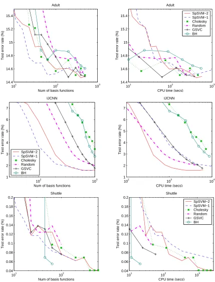
Figures 1 and 2 compare the six methods on six data sets.9 Overall, SpSVM-1 and SpSVM-2 give the best performance in terms of achieving good reduction of test error rate with respect to the number of basis functions. Although SpSVM-2 slightly lags SpSVM-1 in terms of performance in the early stages, it does equally well as more basis functions are added. Since SpSVM-2 is significantly less expensive, it is the best method to use. Since SpSVM-1 is quite cheap in the early stages, it is also appropriate to think of a hybrid method in which SpSVM-1 is used in the early stages and, when it becomes expensive, switch to SpSVM-2. The other methods sometimes do well, but, overall, they are inferior in comparison to SpSVM-1 and SpSVM-2. Interestingly, on the IJCNN and Vehicle data

7. We also tried the method of Bach and Jordan (2005) which uses the training labels, but we noticed little improvement.

8. Note that when the set of basis functions is not restricted, the optimalβsatisfiesλβiyi=max(0,1−yioi).

(9)

101 102 103 14.4 14.6 14.8 15 15.2 15.4

Num of basis functions

Test error rate (%)

Adult

101 102 103

14.4 14.6 14.8 15 15.2 15.4

CPU time (secs)

Test error rate (%)

Adult SpSVM−2 SpSVM−1 Cholesky Random GSVC BH

102 103

1 2 3 4 5 6 7

Test error rate (%)

IJCNN

102 103 104

1 2 3 4 5 6 7

CPU time (secs)

Test error rate (%)

IJCNN SpSVM−2 SpSVM−1 Cholesky Random GSVC BH

101 102

0.04 0.06 0.08 0.1 0.12 0.14 0.16 0.18 0.2

Test error rate (%)

Shuttle

101 102 103

0.04 0.06 0.08 0.1 0.12 0.14 0.16 0.18 0.2

CPU time (secs)

Test error rate (%)

Shuttle SpSVM−2 SpSVM−1 Cholesky Random GSVC BH

(10)

102 103 1 2 3 4 5 6 7

Test error rate (%)

M3V8

102 103 104

1 2 3 4 5 6 7

CPU time (secs)

Test error rate (%)

M3V8 SpSVM−2 SpSVM−1 Cholesky Random GSVC BH

102 103

0.5 1 1.5 2 2.5 3 3.5

Test error rate (%)

M3VOthers

102 103

0.5 1 1.5 2 2.5 3 3.5

CPU time (secs)

Test error rate (%)

M3VOthers SpSVM−2 SpSVM−1 Cholesky Random GSVC BH

101 102 103

11.5 12 12.5 13 13.5 14 14.5 15 15.5

Test error rate (%)

Vehicle

102 103 104

11.5 12 12.5 13 13.5 14 14.5 15 15.5 16

CPU time (secs)

Test error rate (%)

Vehicle SpSVM−2 SpSVM−1 Cholesky Random GSVC BH

(11)

sets, Cholesky, GSVC and BH are even inferior to Random. A possible explanation is as follows: these methods give preference to points that are furthest away in feature space from the points already selected. Thus, they are likely to select points which are outliers (far from the rest of the training points); but outliers are probably unsuitable points for expanding the decision function.

As we mentioned in Section 1, there also exist other greedy methods of kernel basis selection that are motivated by ideas from boosting. These methods are usually given in a setting different from that we consider: a set of (kernel) basis functions is given and a regularizer (such askβk1) is directly specified on the multiplier vectorβ. The method of Bennett et al. (2002) called MARK is given for least squares problems. It is close to the kernel matching pursuit method. We compare

SpSVM-2 with kernel matching pursuit and discuss MARK in Section 5. The method of Bi et al.

(2004) uses column generation ideas from linear and quadratic programming to select new basis functions and so it requires the solution of, both, the primal and dual problems.10 Thus, the basis selection process is based on the sensitivity of the primal objective function to an incoming basis function. On the other hand, our SpSVM methods are based on computing an estimate of the de-crease in the primal objective function due to an incoming basis function; also, the dual solution is not needed.

4. Hyperparameter Tuning

In the actual design process, the values of hyperparameters need to be determined. This can be done using k-fold cross validation. Cross validation (CV) can also be used to choose d, the number of basis functions. Since the solution given by our method approaches the SVM solution as d becomes large, there is really no need to choose d at all. One can simply choose d to be as big a value as possible. But, to achieve good reduction in the classifier complexity (as well as computing time) it is a good idea to track the validation performance as a function of d and stop when this function becomes nearly flat. We proceed as follows. First an appropriate value for dmaxis chosen. For a given choice of hyperparameters, the basis selection method (say, SpSVM-2) is then applied on each training set formed from the k-fold partitions till dmax basis functions are chosen. This gives an estimate of the k-fold CV error for each value of d from 1 to dmax. We choose d to be the number of basis functions that gives the lowest k-fold CV error. This computation can be repeated for each set of hyperparameter values and the best choice can be decided.

Recall that, at stage d, our basis selection methods choose the(d+1)-th basis function from a set ofκrandom basis functions. To avoid the effects of this randomness on hyperparameter tuning, it is better to make thisκ-set to be dependent only on d. Thus, at stage d, the basis selection methods will choose the same set ofκrandom basis functions for all hyperparameter values.

We applied the above ideas on 11 benchmark data sets from (R¨atsch) using SpSVM-2 as the basis selection method. The Gaussian kernel, k(xi,xj) =1+exp(−γkxi−xjk2) was used. The hyperparameters, λandγwere tuned using 3-fold cross validation. The values, 2i, i=−7,· · ·,7 were used for each of these parameters. Ten different train-test partitions were tried to get an idea of the variability in generalization performance. We usedκ=25 and dmax=25. (The Titanic data set has three input variables, which are all binary; hence we set dmax=8 for this data set.)

Table 1 (already introduced in Section 1) gives the results. For comparison we also give the results for the SVM (solution of (1)); in the case of SVM, the number of support vectors (nSV) is the

(12)

number of basis functions. Clearly, our method achieves an impressive reduction in the number of basis functions, while yielding test error rates comparable to the full SVM.

5. Comparison with Kernel Matching Pursuit

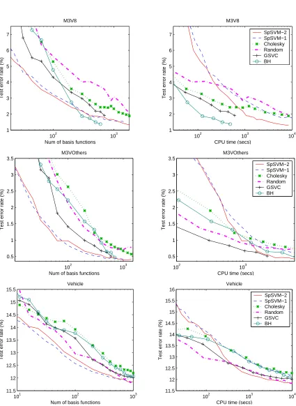
Kernel matching pursuit (KMP) (Vincent and Bengio, 2002) was mainly given as a method of greedily selecting basis functions for the non-regularized kernel least squares problem. As we already explained in Section 3, our basis selection methods can be viewed as extensions of the basic ideas of KMP to the SVM case. In this section we empirically compare the performances of these two methods. For both methods we only consider Basis Selection Method 2 and refer to the two methods simply as KMP and SpSVM. It is also interesting to study the effect of the regularizer term (λkwk2_/_{2 in (1)) on generalization. The regularizer can be removed by setting}λ₌ 0. The original KMP formulation of Vincent and Bengio (2002) considered such a non-regularized formulation only. In the case of SVM, when perfect separability of the training data is possible, it is improper to setλ=0 without actually rewriting the primal formulation in a different form; so, in our implementation we brought in the effect of no-regularization by settingλto the small value, 10−5. Thus, we compare 4 methods: KMP-R, KMP-NR, SpSVM-R and SpSVM-NR. Here “R” and “NR” refer to regularization and no-regularization, respectively.

Figures 3 and 4 compare the four methods on six data sets. Except on M3V8, SpSVM gives a better performance than KMP. The better performance of KMP on M3V8 is probably due to the fact that the examples corresponding to each of the digits, 3 and 8, are distributed as a Gaussian, which is suited to the least squares loss function. Note that in the case of M3VOthers where the “Others” class (corresponding to all digits other than 3) is far from a Gaussian distribution, SVM does better than KMP.

The no-regularization methods, KMP-NR and SpSVM-NR give an interesting performance. In the initial stages of basis addition we are in the underfitting zone and so they perform as well (in fact, a shade better) than their respective regularized counterparts. But, as expected, they start overfitting when many basis functions are added. See, for example the performance on Adult data set given in Figure 3. Thus, when using these non-regularized methods, a lot of care is needed in choosing the right number of basis functions. The number of basis functions at which overfitting sets-in is smaller for SpSVM-NR than that of KMP-NR. This is because of the fact that, while KMP has to concentrate on reducing the residual on all examples in its optimization, SVM only needs to concentrate on the examples violating the margin condition.

It is also useful to mention the method, MARK11 of Bennett et al. (2002) which is closely re-lated to KMP. In this method, a new basis function (say, the one corresponding to the j-th training example) is evaluated by looking at the magnitude (larger the better) of the gradient of the primal objective function with respect toβjevaluated at the currentβJ. This gradient is the dot product of the kernel column containing Ki j and the residual vector having the elements, oi−yi. The compu-tational cost as well as the performance of MARK are close to those of KMP. MARK can also be easily extended to the SVM problem in (1): all that we need to do is to replace the residual vec-tor mentioned above by the vecvec-tor having the elements, yimax{0,1−yioi}. This modified method (which uses our Newton optimization method as the base solver) is close to our SpSVM-2 in terms of computational cost as well as performance. Note that, if we optimize (7) for βj using only a

(13)

101 102 103 14.4

14.6 14.8 15 15.2 15.4

Test error rate (%)

Adult

SpSVM−R SpSVM−NR KMP−R KMP−NR

101 102 103

14.4 14.6 14.8 15 15.2 15.4

CPU time (secs)

Test error rate (%)

Adult

102 103

1 2 3 4 5 6 7 8

Test error rate (%)

IJCNN

102 103 104

1 2 3 4 5 6 7 8

CPU time (secs)

Test error rate (%)

IJCNN

100 101 102

0.05 0.1 0.15 0.2 0.25 0.3

Test error rate (%)

Shuttle

101 102 103

0.05 0.1 0.15 0.2 0.25 0.3

CPU time (secs)

Test error rate (%)

Shuttle

(14)

102 103 1

2 3 4 5 6

Test error rate (%)

M3V8

102 103 104

1 2 3 4 5 6

CPU time (secs)

Test error rate (%)

M3V8

101 102 103

0.5 1 1.5 2 2.5 3 3.5 4

Test error rate (%)

M3VOthers

102 103

0.5 1 1.5 2 2.5 3 3.5 4

CPU time (secs)

Test error rate (%)

M3VOthers

101 102 103

11.5 12 12.5 13 13.5 14 14.5

Test error rate (%)

Vehicle

102 103 104

11.5 12 12.5 13 13.5 14 14.5

CPU time (secs)

Test error rate (%)

Vehicle

(15)

single Newton step, the difference between MARK (as adapted above to SVMs) and SpSVM-2 is only in the use of the second order information.

6. Additional Tuning

We discuss in this section the choice ofκfor SpSVM as well as the possibility of not solving (4) every time a new basis function is added.

6.1 Few Retrainings

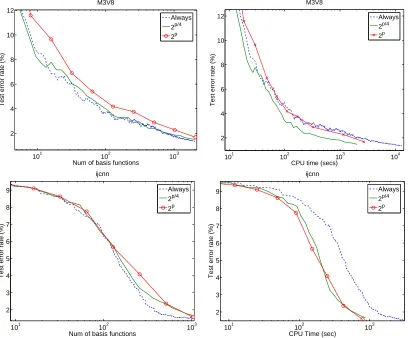
It might be a bit costly to perform the Newton optimization described in Section 2.1 each time a new basis function is added. Indeed, it is unlikely that the set of support vectors changes a lot after each addition. Therefore, we investigate the possibility of retraining only from time to time.

We first tried to do retraining only when|J|=2pfor some p∈N_{, the set of positive integers. It}

makes sense to use an exponential scale since we expect the solution not to change too much when

J is already relatively large. Note that the overall complexity of the algorithm does not change since

the cost of adding one basis function is still O(nd). It is only the constant which is better, because fewer Newton optimizations are performed.

The results are presented in figure 5. For a given number of basis functions, the test error is usually not as good as if we always retrain. But on the other hand, this can be much faster. We found that a good trade-off is to retrain whenever|J|=⌊2p/4⌋for p∈N_{. This is the strategy we}

will use for the experiments in the rest of the paper.

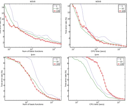
6.2 Influence ofκ

The parameter κis the number of candidate basis functions that are being tried each time a new basis function should be added: we select a random set ofκexamples and the best one (as explained in Section 3.2) among them is chosen. Ifκ=1, this amounts to choosing a random example at each step (i.e. the Random method on figures 1 and 2) .

The influence of κis studied in figure 6. The largerκ is, the better the test error for a given number of basis functions, but also the longer the training time. We found thatκ=10 is a good trade-off and that is the value that we will keep for the experiments presented in the next section.

Finally, an interesting question is how to choose appropriately a good value forκand an efficient retraining strategy. Both are likely to be problem dependent, and even thoughκ=59 was suggested by Smola and Sch¨olkopf (2000), we believe that there is no universal answer. The answer would for instance depend on the cost associated with the computation of the kernel function, on the number of support vectors and on the number of training points. Indeed, the basic cost for one iteration is O(nd)and the number of kernel calculations isκnSV+n: the first term corresponds to

trying different basis function, while the second one correspond to the inclusion of the chosen basis function. Soκshould be chosen such that the kernel computations takes about the same tame as the training itself.

(16)

101 102 103 2

4 6 8 10 12

Test error rate (%)

M3V8

Always 2p/4 2p

101 102 103 104 2

4 6 8 10 12

CPU time (secs)

Test error rate (%)

M3V8

Always 2p/4 2p

101 102 103

2 3 4 5 6 7 8 9

Test error rate (%)

Num of basis functions ijcnn

Always 2p/4 2p

101 102 103 2

3 4 5 6 7 8 9

Test error rate (%)

CPU Time (sec) ijcnn

Always 2p/4 2p

(17)

101 102 103 2

4 6 8 10 12 14

Test error rate (%)

Num of basis functions M3V8

1 10 100

101 102 103 2

4 6 8 10 12 14

CPU time (secs)

Test error rate (%)

M3V8

1 10 100

102 103 2

3 4 5 6 7 8 9

Test error rate (%)

ijcnn

1 10 100

101 102 103 2

3 4 5 6 7 8 9

Test error rate (%)

CPU time (secs) ijcnn

1 10 100

(18)

7. Comparison with Standard SVM Training

We conclude the experimental study by comparing our method with the well known SVM solver,

SVMLight (Joachims, 1999).12 For this solver, we selected random training subsets of sizes from

2−10n,2−9n, . . . ,n/4,n/2,n. For each training set size, we measure the test error, the training time

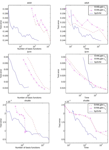
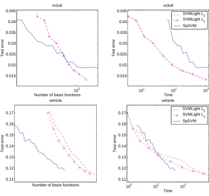
and the number of support vectors. The L2version (quadratic penalization of the slacks) is the one relevant for our study since it is the same loss function as the one we used; note that, when the number of basis functions increases towards n, the SpSVM solution will converge to the L2 SVM solution. For completeness, we also included experimental results of an SVM trained with a L1 penalization of the slacks. Finally, note that for simplicity we kept the same hyperparameters for the different sizes, but that both methods would certainly gain by additional hyerparameter tuning (for instance when the number of basis functions is smaller, the bandwith of the RBF kernel should be larger).

Results are presented in figures 7 and 8. In terms of compression (left columns), our method is usually able to reach the same accuracy as a standard SVM using less than one-tenth the number of basis functions (this confirms the results of table 1).

From a time complexity point of view also, our method is very competitive and can reach the same accuracy as an SVM in less time. The only disappointing performance is on the M3V8 data set. A possible explanation is that for this data set, the number of support vectors is very small and a standard SVM can compute the exact solution quickly.

Finally, note that when the number of basis functions is extremely small compared to the number of training examples, SpSVM can be slower than a SVM trained on a small subset (left part of the right column plots). It is because solving (4) using n training examples while there are only few parameters to estimate is an overkill. It would be wiser to choose n as a function of d, the number of basis functions.

8. Conclusion

In this paper we have given a fast primal algorithm that greedily chooses a subset of the training basis functions to approximate the SVM solution. As the subset grows the solution converges to the SVM solution since choosing the subset to be the entire training set is guaranteed to yield the exact SVM solution. The real power of the method lies in its ability to form very good approximations of the SVM classifier with a clear control on the complexity of the classifier (number of basis functions) as well as the training time. In most data sets, performance very close to that of the SVM is achieved using a set of basis functions whose size is a small fraction of the number of SVM support vectors. The graded control over the training time offered by our method can be valuable in large scale data mining. Many a times, simpler algorithms such as decision trees are preferred over SVMs when there is a severe constraint on computational time. While there is no satisfactory way of doing early stopping with SVMs, our method enables the user to control the training time by choosing the number of basis functions to use.

Our method can be improved and modified in various ways. Hyperparameter tuning time can be substantially reduced by using gradient-based methods on a differentiable estimate of the gen-eralization performance formed using k-fold cross validation and posterior probabilities. Improved methods of choosing theκ-subset of basis functions in each step can also make the method more

(19)

102 103 104 0.144

0.146 0.148 0.15 0.152 0.154 0.156 0.158

Number of basis functions

Test error

adult

101 102 103 0.144

0.146 0.148 0.15 0.152 0.154 0.156 0.158

Time

Test error

adult

SVMLight L 2 SVMLight L

1 SpSVM

103 0.015

0.02 0.025 0.03 0.035 0.04

Test error

ijcnn

102 103 0.015

0.02 0.025 0.03 0.035 0.04

Time

Test error

ijcnn

1 SpSVM

102 103 0.5

1 1.5 2 2.5

x 10−3

Test error

shuttle

101 102 103 0.5

1 1.5 2 2.5

x 10−3

Time

Test error

shuttle

SVMLight L₂ SVMLight L₁ SpSVM

(20)

103 0.015

0.02 0.025 0.03 0.035 0.04 0.045

Test error

m3v8

101 102 103 0.015

0.02 0.025 0.03 0.035 0.04 0.045

Time

Test error

m3v8

1 SpSVM

0.11 0.12 0.13 0.14 0.15 0.16 0.17

Test error

vehicle

100 102 104 0.11

0.12 0.13 0.14 0.15 0.16 0.17

Time

Test error

vehicle

SVMLight L₂ SVMLight L₁ SpSVM

(21)

fective. Also, all the ideas described in this paper can be easily extended to the Huber loss function using the ideas in Keerthi and DeCoste (2005).

Appendix: A Description of Data Sets Used

As in the main paper, let n denote the number of training examples. The six data sets used for the main experiments of the paper are: Adult, IJCNN, M3V8, M3VOthers, Shuttle and Vehicle. For

M3V8 and M3VOthers we go by the experience in (DeCoste and Sch¨olkopf, 2002) and use the

polynomial kernel, k(xi,xj) =1+ (1+xi·xj)9where each xiis normalized to have unit length. For all other data sets, we use the Gaussian kernel, k(xi,xj) =1+exp(−γkxi−xjk2). The values ofγare given below.13 In each case, the values chosen forγandλare ballpark values such that the methods considered in the paper give good generalization performance.

Adult data set is the version given by Platt in his SMO web page: http://www.research.

microsoft.com/∼jplatt/smo.html. Platt created a sequence of data sets with increasing number of examples in order to study the scaling properties of his SMO algorithm with respect to n. For our experiments we only used Adult-8 which has 22,696 training examples and 9865 test examples. Each example has 123 binary features, of which typically only 14 are non-zero. We usedγ=0.05 andλ=1.

The next five data sets are available from the following LIBSVM-Tools page: http://www. csie.ntu.edu.tw/∼cjlin/libsvmtools/datasets/.

IJCNN data set has 49,990 training examples and 91,701 test examples. Each example is

de-scribed by 22 features. We usedγ=4 andλ=1/16.

Shuttle data set has 43,500 training examples and 14,500 test examples. Each example is

de-scribed by 9 features. This is a multiclass data set with seven classes. We looked only at the binary classification problem of differentiating class 1 from the rest. We usedγ=16 andλ=1/512.

M3V8 data set is the binary classification problem of MNIST corresponding to classifying digit

3 from digit 8. The original data set has 11,982 training examples and 1984 test examples for this problem. Since the original test data set could not clearly show a distinction between several closely competing methods, we formed an extended test set by applying invariances like translation and rotation to create an extended test set comprising of 17,856 examples. (This data set can be obtained from the authors.) We usedλ=0.1.

M3VOthers data set is another binary classification problem of MNIST corresponding to

differ-entiating digit 3 from all the other digits. The data set has 60,000 training examples and 10,000 test examples. We usedλ=0.1.

Vehicle data set corresponds to the “vehicle (combined, scaled to [-1,1])” version in the

LIBSVM-Tools page mentioned above. It has 78,823 training examples and 19,705 test examples. Each ex-ample is described by 100 features. This is a multiclass data set with three classes. We looked only at the binary classification problem of differentiating class 3 from the rest. We usedγ=1/8 and λ=1/32.

Apart from the above six large data sets, we also used modified versions of UCI data sets as given in (R¨atsch). These data sets were used to show the sparsity that is achievable using our method; see Table 1 of Section 1 and the detailed discussion in Section 4.

(22)

References

J. Adler, B. D. Rao, and K. Kreutz-Delgado. Comparison of basis selection methods. In Proceedings

of the 30th Asilomar conference on signals, systems and computers, pages 252–257, 1996.

F. Bach and M. Jordan. Predictive low-rank decomposition for kernel methods. In Proceedings of

the Twenty-second International Conference on Machine Learning (ICML), 2005.

K. P. Bennett, M. Momma, and M. J. Embrechts. MARK: A boosting algorithm for heterogeneous kernel models. In Proceedings of SIGKDD’02, 2002.

J. Bi, T. Zhang, and K. P. Bennet. Column generation boosting methods for mixture of kernels. In

Proceedings of SIGKDD’04, 2004.

C. J. C. Burges and B. Sch¨olkopf. Improving the accuracy and speed of support vector learning machines. In Proceedings of the 9thNIPS Conference, pages 375–381, 1997.

O. Chapelle. Training a support vector machine in the primal. Journal of Machine Learning

Re-search, 2005. submitted.

D. DeCoste and B. Sch¨olkopf. Training invariant support vector machines. Machine Learning, 46: 161–190, 2002.

T. Downs, K. E. Gates, and A. Masters. Exact simplification of support vector solutions. Journal of

Machine Learning Research, 2:293–297, 2001.

J. H. Friedman. Greedy function approximation: a gradient boosting machine. Annals of Statistics, 29:1180, 2001.

T. Joachims. Making large-scale SVM learning practical. In Advances in Kernel Methods - Support

Vector Learning. MIT Press, Cambridge, Massachussetts, 1999.

S. S. Keerthi and W. Chu. A matching pursuit approach to sparse Gaussian process regression. In

Proceedings of the 18thNIPS Conference, 2006.

S. S. Keerthi and D. DeCoste. A modified finite Newton method for fast solution of large scale linear svms. Journal of Machine Learning Research, 6:341–361, 2005.

N. Lawrence, M. Seeger, and R. Herbrich. Fast sparse Gaussian process methods: The Informative Vector Machine. In Proceedings of the 15thNIPS Conference, pages 609–616, 2003.

Y. J. Lee and O. L. Mangasarian. RSVM: Reduced support vector machines. In Proceedings of the

SIAM International Conference on Data Mining. SIAM, Philadelphia, 2001.

K. M. Lin and C. J. Lin. A study on reduced support vector machines. IEEE TNN, 14:1449–1459, 2003.

S. G. Mallat and Z. Zhang. Matching pursuits with time-frequency dictionaries. IEEE Transactions

on ASSP, 41:3397–3415, 1993.

(23)

J. A. Meijerink and H. A. van der Vorst. An iterative solution method for linear systems of which the coefficient matrix is a symmetric M-matrix. Mathematics of Computation, 31:148–162, 1977.

E. Osuna and F. Girosi. Reducing the run-time complexity of support vector machines. In

Proceed-ings of the International Conference on Pattern Recognition, 1998.

E. Parrado-Hernández, I. Mora-Jimenéz, J. Arenas-Garc´ıa, A. R. Figueiras-Vidal, and A. Navia-Vázquez. Growing support vector classifiers with controlled complexity. Pattern Recognition, 36:1479–1488, 2003.

J. Platt. Sequential minimal optimization: A fast algorithm for training support vector machines. Technical report, Microsoft Research, Redmond, 1998.

G. R¨atsch. Robust boosting via convex optimization. PhD thesis, University of Potsdam, Department of Computer Science, Potsdam, Germany, 2001.

G. R¨atsch. Benchmark repository. http://ida.first.fraunhofer.de/∼raetsch/.

B. Sch¨olkopf, S. Mika, C. J. C. Burges, P. Knirsch, K. R. Muller, G. Raetsch, and A. J. Smola. Input space vs. feature space in kernel-based methods. IEEE TNN, 10:1000–1017, 1999.

M. Seeger. Low rank updates for the Cholesky decomposition. Technical report, University of California, Berkeley, 2004.

M. Seeger, C. Williams, and N. Lawrence. Fast forward selection to speed up sparse Gaussian process regression. In Proceedings of the Workshop on AI and Statistics, 2003.

A. J. Smola and P. L. Bartlett. Sparse greedy Gaussian process regression. In Proceedings of the

13thNIPS Conference, pages 619–625, 2001.

A. J. Smola and Sch¨olkopf. Sparse greedy matrix approximation for machine learning. In

Proceed-ings of the 17thInternational Conference on Machine Learning, pages 911–918, 2000.

I. Steinwart. Sparseness of support vector machines - some asymptotically sharp bounds. In

Pro-ceedings of the 16thNIPS Conference, pages 169–184, 2004.

T. Thies and F. Weber. Optimal reduced-set vectors for support vector machines with a quadratic kernel. Neural Computation, 16:1769–1777, 2004.

M. E. Tipping. Sparse Bayesian learning and the Relevance Vector Machine. Journal of Machine

Learning Research, 1:211–244, 2001.

P. Vincent and Y. Bengio. Kernel matching pursuit. Machine Learning, 48:165–187, 2002.

M. Wu, B. Sch¨olkopf, and G. Bakir. Building sparse large margin classifiers. In Proceedings of the