Value Function Approximation using Multiple Aggregation for
Multiattribute Resource Management
Abraham George [email protected]
Warren B. Powell [email protected]
Department of Operations Research and Financial Engineering Princeton University
Princeton, NJ 08544, USA
Sanjeev R. Kulkarni [email protected]
Department of Electrical Engineering Princeton University
Princeton, NJ 08544, USA
Editor: Sridhar Mahadevan
Abstract
We consider the problem of estimating the value of a multiattribute resource, where the attributes are categorical or discrete in nature and the number of potential attribute vectors is very large. The problem arises in approximate dynamic programming when we need to estimate the value of a multiattribute resource from estimates based on Monte-Carlo simulation. These problems have been traditionally solved using aggregation, but choosing the right level of aggregation requires resolving the classic tradeoff between aggregation error and sampling error. We propose a method that estimates the value of a resource at different levels of aggregation simultaneously, and then uses a weighted combination of the estimates. Using the optimal weights, which minimizes the variance of the estimate while accounting for correlations between the estimates, is computationally too expensive for practical applications. We have found that a simple inverse variance formula (adjusted for bias), which effectively assumes the estimates are independent, produces near-optimal estimates. We use the setting of two levels of aggregation to explain why this approximation works so well.
Keywords: hierarchical statistics, approximate dynamic programming, mixture models, adaptive learning, multiattribute resources
1. Introduction
• Managing pilots for business jets - The attributes of a pilot include elements such as home city, number of days away from home and the equipment that he is trained to fly. Decisions about pilots can include assigning a pilot to a particular flight, or a decision to send a pilot for training on a new type of aircraft.
• Managing locomotives - The decision to assign a particular locomotive to a particular train has to consider attributes such as the type of locomotive, the number of days until it has to be maintained, its current location and its home maintenance shop.
• Managing a fleet of freight cars - Freight cars have attributes such as location, time until arrival to a destination, loaded or empty status, ownership, and maintenance status.
• Managing a fleet of trucks to move loads - The truck can be described using attributes such as its current location, the home domicile of the driver, the maintenance level and whether it is being driven by a solo driver or a team of two drivers. Decisions include where to move to and whether to move loaded or empty.
• Managing cargo aircraft for the military - We have to decide which aircraft should be assigned to satisfy a particular requirement (a movement of freight or passengers). Choosing the best aircraft requires knowing the value of an aircraft at the destination which depends on the type of aircraft, cargo configuration, whether it is loaded or empty (and if loaded, the load characteristics), and its maintenance status.
• Managing blood inventories - Blood is characterized by blood type, age, location, and whether it has been frozen. New supplies of, and the demand for, blood is random.
All of these are examples of resource allocation problems where a decision has to be made now to act on resources (trucks, jets, locomotives) which will bring about a change in their attributes. Let
a∈
A
be the attribute vector describing a resource now. If we act on the resource, we may produce a resource with attribute a0with value va0. In a dynamic programming setting, the value va0 refers tothe solution of a finite horizon discounted reward dynamic program. In practical applications, we cannot compute va0 exactly, so we resort to Monte Carlo methods where we might observe random
observations ˆva0 and use these to produce a statistical estimate va0 (see Bertsekas and Tsitsiklis
1996 and Sutton and Barto 1998 for an introduction to the techniques of approximate dynamic programming). The problem is that in realistic problems, the attribute space
A
can be extremely large, and we may obtain only a few observations of ˆva0for a particular a0. As a result, the statisticalerror in va0 can be quite large.
One of the standard strategies in approximate dynamic programming is to aggregate the state (attribute) space. Instead of estimating va, we might define an aggregation function G(a) which produces an aggregated attribute a which has fewer outcomes. For example, a five-digit zip code can be aggregated up to a three-digit zip; a numerical attribute can be divided into fewer ranges; or an attribute can be completely ignored. The resulting smaller attribute space produces more observations of each attribute, but at a cost of aggregation error.
we would have to start from scratch if we wished to switch to another application. In fact, simply adding an attribute would require redesigning and refitting the statistical equation. This can be particularly hard when several of the attributes are categorical, and which interact to determine the effect of the attributes on the system. A truck driver might be characterized by his location and his home domicile; the value of a driver at a location depends very much on where he lives.
We are interested in developing a method for estimating the value vaof a resource with attribute
a, making minimal assumptions about the structure of the attribute space. We take advantage of
the fact that for every application with which we are familiar, it is quite easy to design a family of aggregation functions
G
where G(g):A
→A
(g)is an aggregation of the attribute spaceA
. Forex-ample, we can create an aggregation function simply by ignoring an attribute. Aside from assuming the existence of this family of functions, we make no further assumptions about the nature of the attribute space. For example, we do not even require the existence of a metric that would provide a measure of the distance between two attribute vectors, which prevents the use of standard methods such as non-parametric statistics or regression trees.
Aggregation has traditionally been a powerful technique in dynamic programming. A good general review of aggregation techniques is given by Rogers et al. (1991). Aggregation strategies in a dynamic programming setting may be governed by the desire to solve exactly a smaller dynamic program, or by the iterative nature of the algorithms. Techniques range from picking a fixed level of aggregation (Whitt, 1978; Bean et al., 1987; Athans et al., 1995; Zhang and Sethi, 1998; Wang and Dietterich, 2000), or using adaptive techniques that change the level of aggregation as the sampling process progresses (Mendelssohn, 1982; Bertsekas and Tsitsiklis, 1996; Luus, 2000; Kim and Dean, 2003), but which still use a single level of aggregation at any given time (many authors used a fixed level of aggregation to produce a smaller Markov Decision Process (MDP) that can be solved optimally). Tsitsiklis and Van Roy (1996) (see also Bertsekas and Tsitsiklis, 1996) show how value functions can be approximated using a fixed set of features; this strategy encompasses both static and hierarchical aggregation as special cases, but the use of these techniques in our setting is prohibitive because of the extremely large number of values that need to be estimated. Feng et al. (2003) presents a work that identifies state aggregations based on “structural similarity” where states are considered similar if they have similar value estimates or similar sets of successor states, rather than “input similarity” which is typically measured by some distance metric defined over the state space. Bertsekas and Castanon (1989) introduces a creative approach which adaptively clusters states with similar values of residual errors at each iteration, requiring no structure among the states of the system. While we also do not have any structure, we do take advantage of the presence of a family of aggregation functions, and our technique does not require the overhead of solving clustering problems. A nice discussion of aggregation and abstraction techniques in an approximate dynamic programming setting is given in Boutilier et al. (1999).
In this paper, we solve the problem of optimally combining (correlated) value estimates at dif-ferent levels of aggregation in an approximate dynamic programming setting and derive expressions for optimal weights. The result generalizes a well-known result for optimally combining indepen-dent estimates. We point out that the independence assumptions used for deriving the results are true only in idealized regression settings, and not in an approximate dynamic programming setting. The major contribution of this paper lies in finding that an inverse-variance weighting formula (adjusted for bias), which is optimal only when the estimates are independent, proves to be near-optimal even though estimates at different levels of aggregation are not independent. We explain this behavior analytically for the case with two levels of aggregation. We show that if we compute optimal weights (without assuming independence) and compare the results if we do assume inde-pendence, the results are the same for two extremes: when the difference between the aggregate and disaggregate value estimates is very large or very small. We show experimentally that the error for intermediate values is extremely small.
We also show, in the context of a single vehicle routing problem, that our weighting method produces value function estimates that are within five to ten percent of the optimal value functions, outperforming other estimates. The method of weighting a family of aggregate estimates is shown to naturally shift the weight from aggregate to disaggregate estimates as the algorithm progresses. We also demonstrate that this method is easy to implement in large-scale, on-line learning applications that arise in approximate dynamic programming, where it produces much faster convergence (which implies approaching a consistently better solution quality in a fewer number of iterations) than would be produced using a single, static level of aggregation. Further work on this application is explained in detail in Simao et al. (2008).
The paper is organized as follows. In Section 2, we describe a generic approximate dynamic programming technique, which estimates the value functions associated with various states. This section provides an introduction to the context in which our statistical estimation problem arises. The next three sections, however, focus purely on the statistics of aggregation outside of a dynamic programming setting. Section 3 provides a theoretical model of the sampling process and defines bias and variance for aggregated statistics. Then, Section 4 poses the problem of computing optimal weights for combining estimates of values at different levels of aggregation. The problem with this formula is that it is too expensive to use for our problem class. For this reason, we propose a simpler formula that assumes that statistics from different levels of aggregation are independent. In Section 5, we compare the two weighting formulas (with and without the independence assumption) for the special case where there are only two levels of aggregation which allows the optimal weights to be computed analytically. We show theoretically that assuming independent estimates introduces zero expected error at two extremes of the problem. We then show experimentally that ignoring the dependence between the estimates gives results that are very similar. In Section 6, we demonstrate our approximation method in the context of an approximate dynamic programming algorithm for solving a multiattribute resource allocation problem. We use both a single truck problem, which can be solved exactly, as well as a problem of managing a large fleet of trucks. We provide our concluding remarks in Section 7.
2. Approximate Dynamic Programming
allocation problems. Dynamic programming techniques can be applied to solve these problems which are typically modeled as MDPs. Using the notation of Powell (2007), we let St be the state of our system. We also let d∈
D
be a type of a decision, and we let xd =1 if we choose decisiond, and xd=0 otherwise. xt = (xd)d∈D is the vector of decisions that we make at time t. Bellman’s
equation allows us to express the value of being in state St as
V(St) = max xt
[C(St,xt) +E{V(St+1(St,xt,Wt+1))|St}],
where Wt+1 is a random variable representing new information that arrives between t and t+1.
The exact values can be determined using traditional backward dynamic programming techniques such as value iteration and policy iteration. In these methods, the values are computed recursively starting from the final state, making use of the state transition probabilities.
When the state and action spaces become large, as in most real-life stochastic planning prob-lems, it is not practical to enumerate the states to determine their values. In such probprob-lems, compact feature-based representations of the MDP, also called factored MDPs (see Boutilier et al., 2000) can be used to make the problem computationally tractable. Factored MDPs can be represented using a factored state transition model and a reward function that is additive. In these representations, a smaller set of variables (also called features or attributes) are used to describe the state of the system.
Dynamic resource allocation problems span dynamic vehicle routing (Gendreau and Potvin, 1998; Ichoua et al., 2005), where there has been recent interest in the application of approximate dynamic programming for the single vehicle routing problem (Secomandi, 2000, 2001). Powell and Carvalho (1998) uses an approximate dynamic programming algorithm for a fleet management problem, but the attributes of the vehicles were very simple. Powell et al. (2002) uses an approxi-mate dynamic programming algorithm for multiattribute resources, but does not address statistical sampling issues. Spivey and Powell (2004) applies approximate dynamic programming for opti-mizing a fleet of vehicles, using a linear value function approximation that also requires estimating the value of a resource characterized by a vector of attributes. This research estimated the value of a resource at different levels of aggregation, but kept track of the variance of these estimates at each level of aggregation and always used the estimate that provided the smallest variance.
Resource allocation problems can be modeled by letting a∈
A
be an attribute vector (a may consist of categorical and numerical attributes), and by letting Rtabe the number of resources with attribute a. We then let Rt =Rta)a∈A be the resource state vector. This research addresses problemswhere the vector a is large enough that the attribute space
A
becomes too large to enumerate. We develop these ideas in the context of a single entity. If at is the attribute of the entity at time t, thenat is effectively our state variable.
In this section, we describe the basic approximate dynamic programming (ADP) strategy to solve the problem of managing a single resource with multiple attributes, the nomadic trucker. This is a single resource version of the dynamic fleet management problem, where there is a single trucker who needs to move between various locations to cover loads that arise and gains rewards in the process.
this problem would consist of all possible combinations of the attributes of the trucker. We can let the decision be represented by the vector(xd)d∈D, but for a single entity problem, ∑d∈Dxd =1, which means we can also write the problem as choosing a decision d∈
D
. Typically, the set of potential decisions depends on the current state (attributes) of our resource, so we letD
a be the decisions available to a resource with attribute a. We assume that the impact of a decision d on a resource with attribute a is deterministic, and is given by the function a0=aM(a,d).In approximate dynamic programming, we sample the various states by choosing decisions that are locally optimal based on current estimates of the value functions. For example, we could follow a procedure where we choose a decision that maximizes the sum of the one-period rewards and the future value (discounted by factorγ) as follows:
d(a,ω) = arg max d∈Da(ω)
c(a,d,ω) +γvaM(a,d) .
Here, ω represents a sample realization of random information (for example,
D
a(ω) is a sample realization of the decision set), aM(a,d)is the state at the destination and vaM(a,d)the valueassoci-ated with aM(a,d). This model is easily generalized to handle stochastic transitions, but this is not relevant to the focus of this paper.
We outline the steps of a typical approximate dynamic programming algorithm for the nomadic trucker problem in Figure 1. This algorithm has two stages. In the forward pass, we use the current estimates of the optimal value functions to simulate a sample trajectory of the truck. The next state that is visited is determined using a transition function aM(am,dm), as depicted in Equation 2, where the resource in state am undergoes a transformation to state am+1=aM(am,dm) when acted upon by decision dm. Once the end of the time horizon is reached, we perform a backward pass, where we first compute the observations of values of the various states in the current sample path using Equation 3. We point out that the estimates of the future values are discounted by a factorγ. We then use these to update the value estimates, as in Equation 4, and the associated statistics (number of observations and sample variance) of the states that are visited.
There are a number of variations of approximate dynamic programming. One family is known as TD(λ)-learning (see Sutton, 1988; Sutton and Barto, 1998), typically parameterized by an artifi-cial discount factorλ. Using a pure forward pass algorithm is equivalent to TD(0), while another variation follows a policy (determined by the current set of approximations), and then does a back-ward traversal to obtain updates of the estimate of the value of being in each state (this is equivalent to T D(1)). Another popular strategy is Q-learning (see Watkins, 1989), where we estimate the quan-tities Q(a,d)which is the value of being in a state a and making decision d. Since the statistical problem of estimating the value of a state-action pair is, of course, even harder than the problem of estimating the value of being in a state, we have not used this approach. Since Q-learning allows you to determine a decision directly from the Q-factors (rather than solving an optimization problem), it is typically presented as a “model-free” algorithm (that is, one that does not require an explicit model of the transition function), although estimating the Q-factors does require some source that determines the next state given a state and action. All of these methods can be used without an ex-plicit model of the exogenous information process (for example, we do not use a one-step transition function) as long as we have some mechanism for creating the sample realizations.
Step 0. Initialize an approximation for the value function v0
a for all attribute vector states a∈
A
and set n=1 .Step 1. Iteration n:
Step 2. Forward pass: Set m=0 and randomly sample attribute vector am, but fixing the start time at the beginning of the time horizon.
Step 3. Obtain the set of possible decisions,
D
am(ω).Step 4. Solve for the optimal decision, given the current value function estimates.
dm(ω) = arg maxd∈Dam(ω) h
c(am,d) +γvna−1M(a m,d)
i
(1)
Step 5. Evaluate the next state to visit:
am+1 = aM(am,dm) (2) Step 6. If the end of the time horizon (T ) is reached, then set m=m+1 and go to step
3, else go to step 7.
Step 7. Backward pass: For j=m−1,m−2,· · ·,0, update the value function estimates as follows:
ˆ
vnaj = c(aj,dj) +γvˆnaj+1 (3) vanj = (1−α)van−1j +αvˆnaj (4)
Step 8. Let n=n+1. If n<N go to step 1, else for each state a, return the value function vna.
Figure 1: An approximate dynamic programming algorithm using a backward pass for the nomadic trucker problem
visited only a few times. As a result, there can be a high level of statistical noise in our estimates of the value of being in a state.
This section provides the context in which our adaptive learning problem arises. The next three sections consider the general problem of estimating a quantity (the value of a resource with attribute
a) outside of the context of approximate dynamic programming. We assume we have a source of
3. The Statistics of Aggregation
In this section, we investigate the statistics of aggregation by studying a sampling process where at iteration n we first sample the attribute vector a=aˆn. We then use a sample realization of the random information which provides us with an unbiased observation of the value of the resource
ˆ
vn, producing a sequence of observations of (attribute vector, value) pairs. We wish to use this information to produce a statistically reliable estimate of the true value associated with a. The analysis in this section is not done in the context of dynamic programming (which allows us to assume that our observations of values are unbiased). Rather, it is intended as a pure study of the statistics of aggregation.
Our assumption that the observations of values, ˆvn, are unbiased will not be true in a dynamic programming setting, but allows us to focus on the tradeoff between bias and variance.
We begin by defining the following:
N
= The set of indices corresponding to the observations of the attribute vectors and values.S
= A sample of observations(aˆn,vˆn)n∈N.νa= The true value associated with attribute vector a.
Na= The number of observations of attribute vector a given our sample
S
. ˆan= The attribute vector at observation n. ˆ
vn= The observation of the value corresponding to index n. 1{aˆn=a}= 1, if the nth observation is of attribute vector a.
An estimate of νa can be obtained as an average across all the observations of values corre-sponding to a:
va= 1
Nan
∑
∈N ˆvn1{ˆan=a}.
Throughout our presentation, we use the hat notation (as in ˆv) to represent exogenous information,
and bars (as in v) to represent statistics derived from exogenous information.
Consider a case where the attribute vector has more than one dimension, with Ai denoting the number of distinct states that attribute aican assume. The number of values that need to be estimated is∏iAi. Needless to say, as the attribute vector grows, the state space grows exponentially, making it impossible to obtain statistically reliable estimates. One strategy is to resort to aggregation (such as dropping one or more dimensions of a) which can quickly reduce the number of values but introduces structural error. An alternative is to assume a structural property such as separability, which reduces the number of values to be estimated to∑iAi. This has fewer values, but requires that we introduce separability as an approximation. In one of our trucking applications, one attribute is the location of the truck, while a second attribute is the driver’s home domicile. The value of a driver in a location depends very much on his home domicile. Assuming these are independent would introduce significant errors.
In general, aggregation of attribute vectors is performed using a collection of aggregation func-tions, Gg:
A
→A
(g), whereA
(g)represents the gth level of aggregation of the attribute spaceA
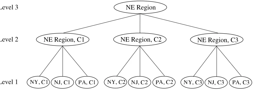
. We define the following:Figure 2: Aggregation of the state space for a multiattribute problem.
G
= The set of indices corresponding to the levels of aggregation.Aggregation can thus be used to create a sequence of state spaces,
A
(g),g=1,2, . . . ,|G
| , with fewer elements than the original state space. This can be better illustrated using the example in Figure 2, where we consider the nomadic trucker problem with the state of the truck defined by two attributes - current location and capacity type. The number of possible states with three locations (NY, NJ and PA), and three capacity types (C1, C2 and C3), is nine at the most disaggregate level. The first-level aggregation function, G(1), involves aggregating the location to the regional level which reduces the number of states to three. The second-level aggregation function, G(2), would be defined as aggregating out the capacity type attribute completely, which leaves us with a single state. As in this example and in the experimental work to follow, it is usually the case that the gth level of aggregation acts on the(g−1)st level.We let εndenote the error in the nth observation with respect to the true value associated with ˆ
an (which, using the notation defined earlier in this section, would be represented usingνaˆn). For
analysis purposes, we assume that the elements of the sequence{εn}
n∈N are independent and
iden-tically distributed, with a mean value of zero. This is, of course, an idealization, but it will help us understand the tradeoffs between structural errors (due to aggregation) and statistical errors. We can express the observed value as follows:
ˆ
vn=νaˆn+εn.
We define the following probability spaces,
Ωa= The set of outcomes of observations of attribute vectors.
Ωε= The set of outcomes of observations of the errors in the values.
Ω= The overall set of outcomes
= Ωa×Ωε.
ω= (ωa,ωε)
We now define the following terms which will be useful in obtaining an estimate of the value associated with the attribute vector a at any level of aggregation:
N
(g)a = The set of indices that correspond to observations of the attribute vector a at the
gth level of aggregation = {n|Gg(aˆn) =Gg(a)}.
Na(g)=
N
(g) a
.
v(ag)= The estimate of the value associated with the attribute vector a at the gth level of aggregation, given the sample,
N
.We can compute the estimate, v(ag), as
v(ag) = 1
Na(g)n∈
∑
N(g) aˆ
vn.
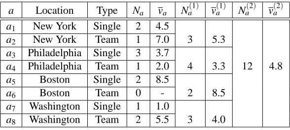
We provide a numerical example to illustrate the idea of forming estimates at different levels of aggregation. Consider the state of a resource to be composed of two attributes, namely, location of the resource and resource type. There are four locations, namely, New York, Philadelphia, Boston and Washington. The type can be Single or Team. Thus, there are eight possible states. We use aggregation functions that aggregate out the type attribute and then the location attribute to obtain three different levels of aggregation. Suppose we have the following observations of state-value
a Location Type Na va Na(1) va(1) Na(2) v(a2)
a1 New York Single 2 4.5
a2 New York Team 1 7.0 3 5.3
a3 Philadelphia Single 3 3.7
a4 Philadelphia Team 1 2.0 4 3.3 12 4.8
a5 Boston Single 2 8.5
a6 Boston Team 0 - 2 8.5
a7 Washington Single 1 1.0
a8 Washington Team 2 5.5 3 4.0
Table 1: Numerical example illustrating the computation of value estimates using aggregation. For example, v(a01)= (7+2)/2=4.5, and v
(1)
a7 = (5+1+6)/3=4.0.
pairs -{(a3,4),(a4,2),(a1,7),(a5,8),(a3,2),(a8,5),(a7,1),(a5,9),(a8,6),(a2,7),(a3,5),(a1,2)}.
We can form estimates of the values of the various states at the different levels of aggregation as illustrated in Table 1.
In order to better understand these two kinds of errors in an aggregation setting, we first letδ(ag) denote the total error in the estimate, v(ag), from the true value associated with attribute vector a:
δ(g)
a = v
(g) a −νa.
An important component of our prediction error will be aggregation bias. Consider our most re-cently observed attribute vector ˆanand some other attribute a, where ˆanand a may aggregate up to the same aggregated attribute at some level g∈
G
, that is, Gg(a) =Gg(aˆn)(for the moment, these are simply two attribute vectors). In our derivations below, it is useful to define a bias term,µna=νaˆn−νa.
We can use this notation to rewrite ˆvnas follows: ˆ
vn = νa+ (νaˆn−νa) +εn
= νa+µna+εn ∀a,n.
We can express v(ag)in terms of its bias and noise components as follows:
v(ag) = 1
Na(g)n∈
∑
N(g) a(νa+µna+εn)
= νa+
1
Na(g)n∈
∑
N(g) aµna
+
1
Na(g)n∈
∑
N(g) aεn
.
We let,
µ(ag) = 1
Na(g)n∈
∑
N(g) aµna,
ε(g)
a =
1
Na(g)n∈
∑
N(g) a.εn.
This enables us to express the total error as follows:
δ(g)
a = µ
(g)
a +ε(ag) (5)
where µ(ag)gives an estimate of the bias between the values of a at the gth level of aggregation and at the disaggregate level. µ(ag)is a random variable that is a function of the set of points sampled.
ε(g)
In an approximate dynamic programming setting, the right tradeoff between statistical and struc-tural errors will change as we collect more observations. Furthermore, we generally do not control the sampling process of the attributes, and we will encounter instances where some regions of the attribute space
A
will be sampled more than others. Although it is common in practice to choose a single level of aggregation that produces the lower overall error, it can be useful to combine esti-mates from several levels of aggregation.4. Combining Estimates
In this section, we propose methods to compute weights to combine value estimates that have been formed from a given set of observations. In the context of ADP, the weights are computed at a given iteration of the algorithm in Figure 1.
We consider a set of estimates,nv(ag),g∈
G
o
, of a value,νa, at different levels of aggregation.
We letσ(ag)denote the population standard deviation associated with the observations used to com-pute v(ag). Breiman (1996) proposes a method called stacked regression which in our setting would be equivalent to combining estimates at different levels of aggregation using
va=
∑
g∈Gw(g)·v(ag),
where w(g) is a set of weights for each level of aggregation. This method ignores the important feature that the best weighting depends on how many times we have observed a particular attribute. We prefer to use the strategy suggested by LeBlanc and Tibshirani (1996) (Section 8), where the weights depend on the attribute:
va=
∑
g∈Gw(ag)·v(ag).
The practical challenge here is that we have to estimate a set of weights(w(ag))for each attribute
a (that we observe). If we use classical regression methods for our applications, this can mean
maintaining hundreds of thousands of regression models. Storing and updating these models is computationally demanding for large industrial applications. In this section, we develop both exact and approximate methods for estimating weights, where our approximation makes the assumption that the estimates v(ag) are independent. Section 5 presents theoretical and experimental arguments supporting the accuracy of the weights when we assume independence (even when the assumption is not even approximately true), which dramatically simplifies the procedure.
4.1 Optimal Weights
We begin by finding the weighting scheme that will optimally combine the estimates at the different levels of aggregation, that is, the weights which give a combined estimate with the least squared deviation from the true value associated with attribute vector a. We can formulate the problem as follows:
min w(ag),g∈G
E
1
2 g
∑
∈Gw(g)
a ·v(ag)−νa
!2
, (6)
subject to:
∑
g∈Gw(ag) = 1. (7)
In a setting where the estimates are unbiased, it is useful to have an affine combination of the estimates (LeBlanc and Tibshirani, 1996, Section 2) since the individual estimates and hence the affine combination are equal to the true value in expectation. Even though this is not necessarily true in a general setting, we choose to retain this constraint.
We state the following proposition for computing the optimal weights that solves the problem formulated in Equations 6-7:
Proposition 1 For a given attribute vector, a, the optimal weights, w(ag), g∈
G
, to combineindi-vidual estimates that are correlated in a hierarchical fashion, are obtained by solving the following system of linear equations in(w,λ):
∑
g∈Gw(ag)E
h
δ(ag)δ (g0) a
i
−λ = 0 ∀ g0∈
G
, (8)∑
g∈Gw(ag) = 1. (9)
If the bias error, µ(ag), is uncorrelated with the random error,ε(ag), then the coefficients of the weights
in Equation 8 can be expressed as follows:
Ehδ(ag)δ (g0) a
i
= Ehµ(ag)µ(g
0)
a
i
+ σ 2
ε
Na(g0)
∀g≤g0 and g,g0∈
G
(10)whereσ2ε denotes the variance of the statistical noise in the observations.
Proof: The proof is given in appendix A. The derivation of Equation 8 involves using the
La-grangian for the problem stated in Equations 6-7 and performing some simple arithmetic on the corresponding first order optimality conditions. Equation 9 is identical to Equation 7 from the opti-mization formulation.
In the remainder of this analysis, our computations will be conditional on a given sequence of observed attribute vectors. In other words, all expectations and probabilities are computed with re-spect to the probability space,Ωε. We prove Equation 10 by simplifying the expressionE
h
δ(g) a δ
(g0) a
i
For the case where g=0, we can use the result, E
h
µ(a0)µ(g
0)
a
i
=0 (which follows from the
property: µ(a0)=0), to further simplify (10) and obtain the following result:
Ehδ(a0)δ (g0) a
i
= σ
2
ε
Na(g0)
. (11)
We refer to the optimal weighting scheme as WOPT.
4.2 An Approximation Assuming Independence
It is a well-known result in statistics that if the estimatesnv(ag),g∈
G
o
were independent and unbi-ased, then the optimal weights would be given by
w(ag) =
1
σ(g) a
2 /Na(g)
∑
g0∈G
1
σ(g0)
a
2 /Na(g0)
−1
. (12)
We can obtain this result from proposition 1 as follows. If we assume that the estimates
n
v(ag),g∈
G
o
are independent and unbiased, then the cross-terms in Equation 8 disappear, leav-ing behind the followleav-ing modified relation:
w(ag)E
δ(ag)
2
−λ = 0 ∀ g∈
G
. (13)Solving Equations 13 and 9 gives us weights that are inversely proportional to the expected squared
errors,Eδ(ag)
2
. For the case of independent, unbiased estimates,Eδ(ag)
2
is identical to the
variance,σ(ag)
2 /Na(g).
Solving the system of equations in Proposition 1 can be computationally expensive since in practice, there may be hundreds of thousands of models. For practical solutions, it will be useful to have an expression along the lines of Equation 12 for computing the weights, even though neither of the conditions (independence and absence of bias) holds true for estimates that arise from aggre-gation due to structural errors introduced in the process of aggreaggre-gation. In order to adapt the simpler formula in (13) to the aggregation setting while acknowledging the bias, we first define:
µ(ag)= Expected bias in the estimate, v(ag)
= Ehv(ag)−νa
i
.
For biased estimates, the total squared error can be expressed as the sum of bias and variance components, provided the bias and variance are independent of each other (Hastie et al., 2001, p. 24):
Eδ(ag)
2
= σ
(g) a
2 Na(g)
+µ(ag)
2
We use this relation to modify the weights as follows:
w(ag)= 1
σ(g) a
2
Na(g)
+µ(ag)
2
∑
g0∈G
1
σ(g0) a
2
Na(g0)
+µ(ag0)
2
−1
∀ g∈
G
. (15)We call this weighting scheme, WIND.
4.3 Weighting by Inverse Mean Squared Errors
In the more realistic setting where the exact values of the parameters involved in the computation of weights as in Equation 15 are unknown, we propose using the plug-in principle (see, for example, Efron and Tibshirani 1993, chapter 4) where we use statistical estimates of the bias and variance to produce approximations of the weights. We first compute estimates of the bias and the variance using
s(ag)
2
= The sample variance of the observations corresponding to the estimate v(ag)
= 1
Na(g)−1n∈
∑
N(g) a
ˆ
vn−v(ag)
2 .
˜µ(ag) = An estimate of the bias in the estimated value (v(ag)) from the true value
= v(ag)−v(a0).
The approximate weights on the estimates at different levels of aggregation are inversely propor-tional to the estimates of their mean squared deviations (obtained as the sum of the variances and the biases) from the true value:
w(ag) =
1
s(ag)
2
Na(g)
+˜µ(g)
2
a
∑
g0∈G
1
s(ag0)
2
Na(g0)
+˜µ(g0)
2 a −1
∀ g∈
G
. (16)We refer to this formula as weighting by inverse mean squared errors (WIMSE). In the event that
Na(g)is too small or zero (which can happen in the early iterations and/or at the more disaggregate levels), it is difficult to form meaningful estimates of the variance and bias. In such a situation, we set the corresponding weight to zero.
Equation 16 is very easy to calculate even for large scale applications where we may observe hundreds of thousands of attributes. However, it produces the best results only when the estimates of values at different levels of aggregation are independent, an assumption that we cannot expect to hold true. In the next section, we present theoretical and experimental evidence supporting the claim that the error introduced from this assumption is negligible.
5. The Case for Assuming Independence
In this section, we justify our decision to ignore the dependence between the estimates from hier-archical aggregation, while combining them to form an improved estimate. We discuss the special case where we combine estimates from only two levels of aggregation, which enables us to obtain simple expressions for computing the various parameters. We assume that the statistical noise is independent of the attribute vector sampled and also that we know the probability distributions of the sampling of the attribute vectors and their values. These assumptions enable us to solve the optimality equations to obtain a solution explicitly. In Section 5.1, we analytically compare the two sets of equations (with and without assuming independence) for computing optimal weights. We provide an experimental comparison of the two methods, demonstrating the similarity in results, in section 5.2.
5.1 Analytical Comparison
For the two-level problem, we can obtain the optimal weights (WOPT) by solving the following system of equations:
E
δ(a0)2
w(a0)+E
h
δ(a0)δ (1) a
i
w(a1)−λ = 0, Ehδ(a0)δ
(1) a
i
w(a0)+E
δ(a1)2
w(a1)−λ = 0,
w(a0)+w(a1) = 1,
w(a0),w(a1) ≥ 0.
Since we are concerned with computing the weights for a particular attribute vector, we drop the index a in the following analysis. We obtain the value of w(0)as,
w(0) =
E
δ(1)2 −E
h
δ(0)
δ(1)i
E
δ(0)2
+E
δ(1)2
−2Ehδ(0)δ(1)i
. (17)
By assumption, the estimate at the disaggregate level is unbiased, that is, µ(0)=0. We let
µ2=Ehµ(1)2idenote the expected value of the square of the bias term at the aggregate level. Using Equations 10 and 11, we may write,
Ehδ(0)δ(1)i = σ 2
ε
N(1),
E
δ(0)2
= σ
2
ε
N(0),
E
δ(1)2
= Ehµ(1)2
i
+Ehε(1)2i
= µ2+ σ 2
ε
These results enable us to rewrite Equation 17 for computing the weights on the disaggregate esti-mate using the WOPT scheme (which we denote as wopt) as follows:
wopt = 1
1+N1(0) −
1
N(1) σ2
ε
µ2
. (18)
The competing scheme, WIND, assumes independence of the estimates. The weights at the disaggregate level are obtained using the formula:
wind = 1+ 1
N(1)
σ2
ε
µ2
1+ 1
N(0)+N1(1) σ2
ε
µ2
. (19)
We denote by ˜vopt and ˜vind the estimates computed using the two weighting schemes. ˜
vopt = woptv(0)+ (1−wopt)v(1),
˜
vind = windv(0)+ (1−wind)v(1).
We can write the difference between the estimates of the value obtained with and without the inde-pendence assumption as∆=v˜opt−v˜ind=∆w·∆v, where∆w=wopt−wind and∆v=v(0)−v(1). The following proposition establishes that∆is small under certain conditions.
Proposition 2 (i) limµ→0E[∆] =0, (ii) limµ→∞∆=0, (iii) limσ2→0∆=0. Proof:
(i) As µ→0, wopt =0 and wind=N(0)/ N(0)+N(1). wind attains a maximum value of 1/2 when
N(0)=N(1), but that would imply that v(0)=v(1)⇒∆v=0. At the other extreme, if N(0)=0, then
wind=0⇒∆w=0. For intermediate values of N(0), it is no longer true that the random variable∆v will always be zero (for statistical reasons), but we can show that its expectation will be zero using
E[∆] = E{E[∆|
N
]},E[∆|
N
] = E"
∆v
N(0) N(0)+N(1)|
N
#
= E[∆v]
N(0) N(0)+N(1)
= 0.
Since µ2=0,E[∆v] =0 and Equation 20 follows.
(ii) As µ→∞, wind→wopt→1, which can be easily obtained by applying the appropriate limits in Equations 18 and 19. This is intuitive since with very high bias, the best strategy is to put all the weight on the most disaggregate level. As a result,∆w→0.
(iii) As the variance goes to zero, w(ind)→w(opt)that again implies∆
w→0.
Aggregate cell 1
Aggregate cell 2
Aggregate cell 3
a
a
v
1 2 3 4 5 6 7 8 9 10
0
a V
1
a V
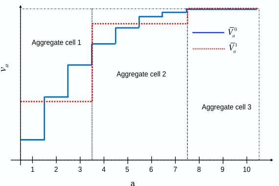
Figure 3: A piecewise constant function with its aggregate approximation. Estimates of values of each attribute vector are computed at both the aggregate and disaggregate levels. A weighted averaging is done to improve the estimates.
5.2 Experimental Results
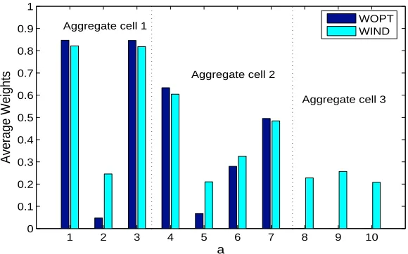
In this section, we analyze the estimation of functions characterized by known parameters (which effectively requires that we know the actual function) in order to demonstrate the effectiveness of the optimal weighting strategy, as well as to serve as a benchmark for the strategy which assumes independent estimates at different levels of aggregation. We observe that the weights given by either method (Equations 18 and 19) are functions of the bias in the value at the aggregate level, the variance of the statistical noise in the observation of the values and the number of observations at either level. In order to compare the values of the weights from the competing strategies, we create scenarios with different combinations of the parameters that would produce significant changes in the weights. We then analyze how the variations in the weights given by WOPT and WIND affect the actual function estimates computed using the two schemes.
1 2 3 4 5 6 7 8 9 10 0
0.1 0.2 0.3 0.4 0.5 0.6 0.7 0.8 0.9 1
a
A
ve
ra
g
e
W
e
ig
h
ts
Aggregate cell 1
Aggregate cell 2
Aggregate cell 3 WOPT WIND
Figure 4: Comparison of the weights over the function domain
We have illustrated the difference in the weights produced by the two strategies, but less obvious is the difference in the estimates of the underlying function. In order to compare the two schemes, we developed a measure of the degree to which a weighting strategy reduced the variance of an estimate. We define the following:
˜
vsa = The value of the attribute vector a as estimated by strategy s.
εs = The sum of squared errors as estimated by strategy s.
=
∑
a∈A
(v˜sa−νa)2
εG = The sum of squared errors using the static aggregation strategy which treats the function as a constant over its domain.
θs = The performance measure for strategy s.
= 1− ε s
εG.
θsmeasures the degree of variability explained by a particular weighting strategy relative to using a single constant which can be thought of as a default strategy where all observations are aggregated together.θsis analogous to an R2measure commonly used in statistics.
A major factor in the performance of a weighting strategy is the relative size of the structural variation compared to the statistical noise. For this purpose, we define an index,ρ, that measures the ratio of the noise to the bias.
Figure 5 compares the performances of the two weighting strategies for three levels of noise. We observe that the performance of WOPT and WIND are almost identical even though there were situations where the weights given by the two schemes were significantly different. The similarity in the function estimates from the two strategies is explained by the analysis in Section 5.1.
0 10 20 30 40 50 60 70 80 90 100 0
0.1 0.2 0.3 0.4 0.5 0.6 0.7 0.8 0.9 1
Number of observations
P
e
rf
o
rm
a
n
ce
m
e
a
su
re
(
θ
s )
ρ = 5
ρ = 2
ρ = 1
ρ = 1 WOPT
ρ = 1 WIND
ρ = 2 WOPT
ρ = 2 WIND
ρ = 5 WOPT
ρ = 5 WIND
Figure 5: Comparison of the performance, as measured byθs, of WOPT and WIND in estimating the piecewise constant function
0 1 2 3 4 5 6 7 8 9 10
0.4 0.5 0.6 0.7 0.8 0.9 1
Average number of observations per disaggregate cell
P
e
rf
o
rm
a
n
ce
m
e
a
su
re
(
θ
s )
Random
Concave non−monotone
Concave
Sinusoidal Linear
2 overlapping lines denotingθs for WOPT (solid line) & WIND (dashed line)
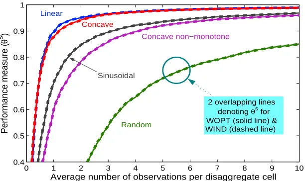
Figure 6: Comparison of WOPT and WIND for various function types using expected values of weights. The graph shows the average performance measure (θs) over 1000 samples for a moderate value ofρ=2. WOPT is represented using solid lines and WIND, with dashed lines - the two are virtually indistinguishable.
6. Experiments in an ADP Application
We implemented the hierarchical weighting strategy in the approximate dynamic procedure for solving the nomadic trucker problem described in Section 2. In Section 6.1, we describe the specifics of the problem instances that we consider. We also state the competing strategies that we compare in the experiments that follow. We then proceed to show the effectiveness of our hierarchical weighting scheme using two sets of experiments. In Section 6.2, we report on experiments where the discount factor is set to zero. In this case, the observations of values are unbiased, since they do not involve the estimates of values of future states. In Section 6.3, we present the results of experiments with positive discount factors. We have made available a collection of data sets used in these experiments on the following webpage - http://castlelab.princeton.edu/. Finally, in Section 6.4, we provide experimental results from applying our techniques on an industrial strength problem.
6.1 Experimental Design
We consider a problem where we specify the state of the truck using three attributes, namely, the current location, the day of week and the number of days away from home. The problem is rich enough to offer interesting opportunities for hierarchical aggregation, but small enough that we can solve the problem to obtain the exact solution.
The decisions are to be made over a finite time horizon of 21 time periods. The location attribute can be represented at two degrees of resolution - regions (eastern Pennsylvania, northern New Jer-sey) or geographical areas (Northeast, Midwest and so on). There are 50 locations at the region level which can be aggregated to 10 geographical areas.
The major contributor to the stochastic nature of the nomadic trucker problem is the uncer-tainty in the availability of loads in any particular location to be moved to other locations. The probability that a load is available to be moved from one location to another is dependent on the origin-destination pair. Another factor that influences the load availability is the day of week. Loads are more likely to appear during the beginning of the week (Mondays) and towards the end (Fri-days). We use a probability distribution whereby the load availability dips during the middle of the week and is lower over the weekends. We introduce further uncertainty into the problem by allowing the one-period contributions to be moderately noisy.
The final attribute that we consider is the number of days that the driver is away from home. There is a penalty that we impose on moves that keep the driver away from his home domicile, which is a quadratic function of the number of days away from home. In order to keep the state space manageable (so we can obtain optimal solutions), we cap the number of days away from home at 12.
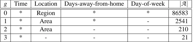
In Table 2, we list the aggregations that we use for the problem and the number of attribute states at each level of aggregation. For example, at aggregation level 1, the location attribute is aggregated from 50 regions to 10 geographical areas. We aggregate out the day-of-week attribute and retain the days-away-from-home attribute. Adding in the factor for 21 time periods, we have a total of 2541 possible states. The apparent discrepancy in the size of the state space at levels 0 and 1 arises because the days-away-from-home attribute is always set to 0 for the location corresponding to the home of the driver, while for all the other locations it can be any number from 1 to 12.
g Time Location Days-away-from-home Day-of-week |
A
|0 * Region * * 86583
1 * Area * - 2541
2 * Area - - 210
3 * - - - 21
Table 2: Aggregations for the multiattribute nomadic trucker problem. A ‘∗’ corresponding to a particular attribute indicates that the attribute is included in the attribute vector, and a ‘−’ indicates that it is aggregated out.
our aggregation strategies in the approximate dynamic programming algorithm outlined in Figure 1. The value function estimate in Equation 1 is obtained as a weighted sum of the value estimates at various levels of aggregation:
vna−10 =
∑
g∈G
w(ag0),n−1v (g),n−1
a0 where a0=aM(a,d)∀d∈
D
awhere w(ag0),n−1denotes the weight, at iteration(n−1), on the estimate of the value of attribute vector a0at the gth level of aggregation.
The methods that we compare use the following sets of weights:
1. Static Aggregation:
w(ag0),n−1 =
1 if g is the fixed level of aggregation, 0 otherwise.
2. Dynamic Aggregation (MINV):
w(ag0),n−1 =
(
1 if g=arg ming0∈G
s(ag00),n−1
2
0 otherwise.
3. WIMSE: w(ag0),n−1is computed using Equation 16.
Equation 4 is replaced by a series of equations for updating the value function estimates at all the levels of aggregation corresponding to the currently visited attribute vector:
For methods 2 and 3, we point out that the chosen level of aggregation and the weights on the estimates at different levels are dynamic in nature, in that they change with each iteration. This is brought out in the sections that follow.
The performance measure that we use for these experiments is based on the deviation of the value function approximations from the optimal value functions which can be obtained using a traditional backward dynamic programming algorithm such as value iteration. We first define
pa = The steady state probability of being in state (equivalent to, in this situation, attribute vector) a.
Na = The number of observations of or visits to state a.
νa = The true value associated with state a. ˜
vsa = The value function approximation for state a estimate computed using strategy s.
Using these we may define the following performance measures:
E1s = Error measure based on steady state probabilities, that is, a stationary dis-tribution
= ∑a∈Apa(v˜
s a−νa)
∑a∈Apaνa
×100%. (21)
E2s = Error measure based on the number of visits to each state
= ∑a∈ANa(v˜
s a−νa)
∑a∈ANaνa
×100%. (22)
6.2 Experiments on Myopic Data Sets
We first analyze the ability of our proposed method to make estimates from a purely statistical perspective. For this purpose, we maintain a zero discount factor, which means that the downstream values of the states are ignored while making the decisions at any time period. Instead the decisions are based on the one-period rewards alone. Using a discount factor of zero eliminates the bias that is introduced in the ADP procedure, which implies that the errors in the estimates are purely due to the noise in the observations. We compare the different estimation techniques in Table 3 where we tabulate the E2s values (as computed using Equation 22) for several problem instances. The static aggregation strategies for g=0,1 & 2 are denoted as Disaggregate, Aggregate1 and Aggregate2 respectively. We observe that WIMSE demonstrates lower errors than the other techniques.
6.3 Experiments on Non-myopic Data Sets
Problem # Disaggregate Aggregate1 MINV WIMSE
1 6.89 0.07 18.06 0.06 7.84 0.13 5.54 0.08
2 9.47 0.07 18.39 0.12 11.99 0.28 7.88 0.09
3 2.92 0.04 17.81 0.07 4.04 0.07 2.95 0.04
4 5.74 0.08 18.06 0.09 8.02 0.16 5.56 0.07
5 2.70 0.05 17.25 0.07 3.27 0.11 2.44 0.05
6 5.52 0.09 17.50 0.09 7.26 0.10 5.10 0.10
Table 3: Comparison of techniques for different problem instances (Disaggregate: g=0, Aggre-gate1: g=1). The performance measure used for each of the methods is the percentage deviation from optimality. Figures in italics denote the standard deviations of the terms to the left.
0 2 4 6 8 10 12
0 0.1 0.2 0.3 0.4 0.5 0.6
Number of observations per state
A
v
e
ra
g
e
w
e
ig
h
ts Disaggregate
Aggregate1 Aggregate2
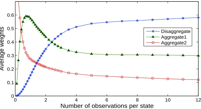
Figure 7: Average weights using hierarchical aggregation. (Disaggregate: g=0, Aggregate1: g=
1, Aggregate2: g=2).
very slowly. This behavior primarily reflects attributes with very low bias where the weight on the aggregate level will always remain fairly high.
0 1 2 3 4 5 6 7 8 9 10 0 5 10 15 20 25 30
Number of iterations (x 105)
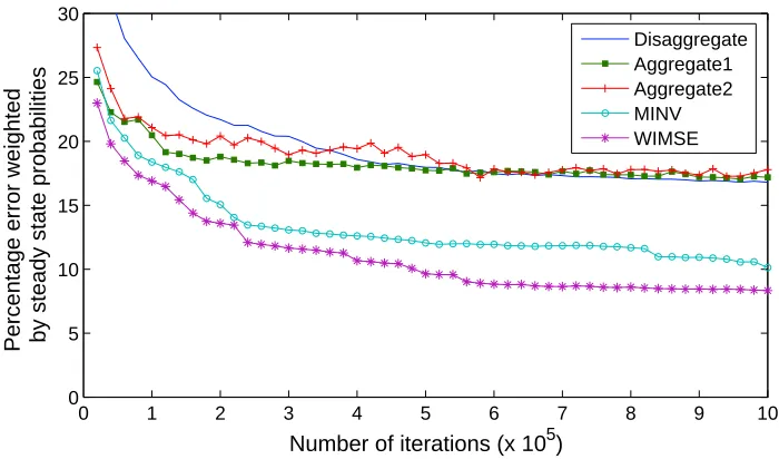
P e rc e n ta g e e rr o r w e ig h te d b y s te a d y s ta te p ro b a b ili ti e s Disaggregate Aggregate1 Aggregate2 MINV WIMSE
Figure 8: E1svalues as a function of the number of observations.
0 1 2 3 4 5 6 7 8 9 10 0
5 10 15
Number of iterations (x 105)
P e rc e n ta g e e rr o r w e ig h te d b y n u m b e r o f v is it s Disaggregate Aggregate1 Aggregate2 MINV WIMSE
Figure 9: E2svalues as a function of the number of observations.
Figure 9 shows the relative performance of the various schemes with respect to the errors weighted by the number of visits to the various states (Es
2 values). This error measure gives an
Problem # Iterations Disaggregate Aggregate1 MINV WIMSE
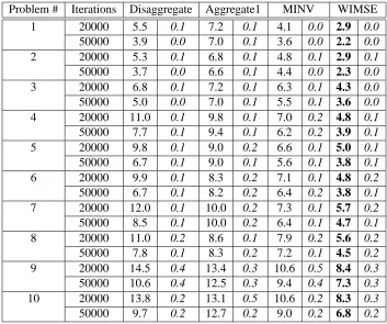
1 20000 5.5 0.1 7.2 0.1 4.1 0.0 2.9 0.0
50000 3.9 0.0 7.0 0.1 3.6 0.0 2.2 0.0
2 20000 5.3 0.1 6.8 0.1 4.8 0.1 2.9 0.1
50000 3.7 0.0 6.6 0.1 4.4 0.0 2.3 0.0
3 20000 6.8 0.1 7.2 0.1 6.3 0.1 4.3 0.0
50000 5.0 0.0 7.0 0.1 5.5 0.1 3.6 0.0
4 20000 11.0 0.1 9.8 0.1 7.0 0.2 4.8 0.1
50000 7.7 0.1 9.4 0.1 6.2 0.2 3.9 0.1
5 20000 9.8 0.1 9.0 0.2 6.6 0.1 5.0 0.1
50000 6.7 0.1 9.0 0.1 5.6 0.1 3.8 0.1
6 20000 9.9 0.1 8.3 0.2 7.1 0.1 4.8 0.2
50000 6.7 0.1 8.2 0.2 6.4 0.2 3.8 0.1
7 20000 12.0 0.1 10.0 0.2 7.3 0.1 5.7 0.2
50000 8.5 0.1 10.0 0.2 6.4 0.1 4.7 0.1
8 20000 11.0 0.2 8.6 0.1 7.9 0.2 5.6 0.2
50000 7.8 0.1 8.3 0.2 7.2 0.1 4.5 0.2
9 20000 14.5 0.4 13.4 0.3 10.6 0.5 8.4 0.3
50000 10.6 0.4 12.5 0.3 9.4 0.4 7.3 0.3
10 20000 13.8 0.2 13.1 0.5 10.6 0.2 8.3 0.3
50000 9.7 0.2 12.7 0.2 9.0 0.2 6.8 0.2
Table 4: Comparison of techniques for different instances of the nomadic trucker problem. Two higher levels of aggregation are also used in the problem, but omitted from the tables, as they give inferior results. Figures in italics denote the standard deviations of the terms to the left.
Here again, WIMSE is found to consistently outperform the remaining techniques, producing error values that are much lower.
We now compare the various techniques for several problem instances. The major parameters that are varied to obtain the different problem sets are the discount factor, the probability distribution of the load availability at the various locations and the level of uncertainty in the contributions resulting from choosing a particular decision. We used discount factors of 0.80, 0.90 and 0.95, three different load probability distributions and two levels of uncertainty in the rewards. The E2s values for these problem instances are tabulated in Table 4. Here again, WIMSE outperforms all the other schemes consistently, irrespective of the number of iterations.
6.4 Experiments with a Fleet of Trucks
all of these problems). Let
Ra = The number of resources with attribute a.
R = (Ra)a∈A
D
= The set of different decision types that can be used to act on a resource (e.g., moving from one location to another, repairing a vehicle).xad = The number of times we act on a resource with attribute a using a decision of type d∈
D
.x = (xad)a∈A,d∈D
cad = The contribution generated by xad.
For problems with moderately complex attribute vectors, we have found that we can obtain high quality solutions using dynamic programming approximations by solving (at iteration n) approxi-mations of the form,
˜
Vn(Rn) =max
x
∑
a∈Ad
∑
∈Dcadxad+
∑
a0∈Avna−10 Rxa0(x)
!
(23)
subject to,
∑
d∈Dxad = Rna ∀a∈
A
, (24)Rxa0 =
∑
a∈Ad
∑
∈Dδa0xad, (25)
xad ≥ 0. (26)
This is a fairly basic model, but it is enough to illustrate the application (for a more complete description, see Spivey and Powell 2004). Problem 23 - 26 is a linear program, and returns a dual variable that we denote ˆvna for the resource constraint in Equation 24. In a real application, the attribute space
A
is large enough that we do not generate Equation 24 for each a∈A
. Instead, we might generate the equation only if Rna>0 (for example). We can then update our value function approximation usingvan= (1−αn)van−1+αnvˆna.
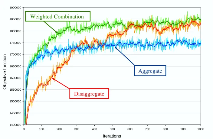
The problem we encounter, just as in the earlier sections, is that real problems might have attribute spaces with several million elements, and yet we can only run a few hundred iterations of the al-gorithm. Many of the attributes are never sampled, while others will have only a few observations. A small handful may receive dozens of observations. As a result, the statistical reliability of the approximations vnacan be quite low. The standard technique is to estimate the values at some aggre-gate level that trades off between the statistical reliability and cost of bias introduced by aggregation. The right level of aggregation depends not only on the specific attribute (some are sampled more often than others) but also on the number of iterations we have run the algorithm.
1400000 1450000 1500000 1550000 1600000 1650000 1700000 1750000 1800000 1850000 1900000
0 100 200 300 400 500 600 700 800 900 1000
Iterations
O
b
je
c
ti
v
e
f
u
n
c
ti
o
n
Weighted Combination
Aggregate
Disaggregate
Iterations
O
b
je
c
ti
v
e
f
u
n
c
ti
o
n
Figure 10: Comparison of using a single level of aggregation (aggregate and disaggregate) against a weighted aggregation strategy for optimizing a fleet of trucks.
of the driver (out of 100 regions), the driver’s home domicile (out of 100 regions), and whether the driver was a single driver employed by the company, a contract driver, or a team (two drivers working together). At the most disaggregate level, the attribute space consisted of 30,000 elements. We considered an aggregate level which captured only the location of the driver (100 elements) and a hierarchical strategy that used a weighted estimate across four levels of aggregation.