Photovoltaic Power Control Using Fuzzy Logic and Fuzzy Logic Type 2 MPPT Algorithms and Buck Converter

(1)

Photovoltaic Power Control Using Fuzzy Logic and Fuzzy Logic Type 2

MPPT Algorithms and Buck Converter

Bachar Meryem

*

, Naddami Ahmed, Fahli Ahmed

Department of Electrical Engineering, Hassan First University, Settat, Morocco

Received 13 March 2019; received in revised form 22 April 2019; accepted 25 May 2019

Abstract

This work presents the analysis, design, simulation and hardware implementation of the classical Fuzzy Logic

(FL) and the proposed Fuzzy Logic Type 2 (FLT2) MPPT techniques for standalone PV System. FL and FLT2

MPPT algorithms are simulated via MATLAB/ Simulink and implemented via LabVIEW software and CompactRio

hardware, in different climatic conditions. Also, they are compared to the Incremental Conductance (InC) MPPT

algorithm, one of the most common used MPPT techniques. The studied system consists of PV array, DC/DC

converter, MPPT controller, batteries and load. The PV array is connected to the DC / DC buck converter that works

based on the output pulses of the MPPT controller to make the PV system operates at the Maximum Power Point

(MPP). Thereafter, based on the simulations and the experimental results, a comparison is made to be useful for

MPPT designers and researchers in this area.

Keywords: photovoltaic panel, fuzzy logic, fuzzy logic type 2, matlab/simulink

1. Introduction

Solar energy is a renewable, non-polluting and economical source of energy which allows obtaining electricity from the

solar irradiation using Photovoltaic (PV) cells [1, 2]. Despite its advantages, solar energy has a remarkable disadvantage. One

of the most relevant problems is that solar energy is intermittent. Therefore, the power produced by PV panels is influenced by

the climatic conditions (irradiation and temperature) and the load impedance [3, 4]. Generally, the intersection of the load and

PV panel characteristics is too far from the MPP, thus, it is important to insert a DC/DC converter, between the load and the PV

source, for the impedance matching [5]. Maximum Power Point Tracking (MPPT) Algorithms are used for the pursuit of MPP

in different climatic conditions [6], by adjusting the duty cycle of the DC/DC converter. Generally, the system consists of a PV

array, a DC/DC converter, a load and finally batteries. Nowadays, several techniques of MPPT exist such as Perturb and

Observe (P&O) [7, 8], Incremental Conductance (InC) [5, 9], Constant Voltage (CV), Open Circuit Voltage (OCV), and Fuzzy

logic (FL) [10-12]. MPPT algorithms can be distinguished by operating principle, performance, complexity, response time,

cost and more.

The classic Fuzzy Logic (FL), introduced in 1965 by Lotfi Zadeh, allows the representation and processing of imprecise

knowledge based on linguistic terms. It relies on human reasoning to convert a linguistic command into an automatic command

to control complex systems [13, 14]. Fuzzy Type 2 (FLT2) [15], the proposed MPPT technique, is based on FL. It supports

uncertainties using three-dimensional membership functions.

*Corresponding author. E-mail address: meryem.bachar@gmail.com

(2)

In this work, the authors present a comparative study of three MPPT Algorithms (Fuzzy Logic, Fuzzy Logic Type 2 and

Incremental Conductance). MATLAB/Simulink environment is used for simulation studies and LabView Software for

experimental tests.

This paper is organized as follows: Section II explains the operating principle of a photovoltaic cell and gives the I-V and

P-V characteristics of the studied PV array. Section III deals with DC/DC converters and focuses on the DC/DC Buck

Converter, used in this paper. Section IV studies the role of MPPT algorithms and explain FL and FLT2 MPPT Algorithms.

Section V presents the simulation results of the photovoltaic system with FL, FLT2, and InC algorithms and gives a

comparison of them. Finally, Section VI presents the experimental results of the three studied Algorithms by using LabVIEW

software and CompactRio Hardware.

2. Photovoltaic Module

In order to study the behaviour of Photovoltaic cell, we can model it by an electric circuit, as shown in Fig. 1. PV cell

usually consists of an Iph current generator, which models the conversion of light radiation into electricity, a diode D which

represents the PN junction, a parallel resistor Rsh and a series resistor Rs [16, 17].

Fig. 1 Electric circuit of PV cell

The current generated by the photovoltaic cell is calculated by Eq. (1):

ph D sh

I I I I (1)

Eq. (1) can be rewritten by Eq. (2) [18]:

0 s sh sh V IR R q s ph V IR

I I I e

R            _     _ _     (2)

The terms Iph, I0, q, A, K, T are the photodiode current, the inverse saturation current, the electron charge, the ideality factor of

the PN junction, the Boltzmann constant and the temperature of PV cell, respectively.

3. DC/DC Buck Converter

Fig. 3 DC/DC Buck Converter

A DC/DC converter is used to convert a DC input voltage to a modified DC output voltage [20]. Currently, several

(3)

which allows for a lowered voltage, is used. It usually consists of a switch, a diode, a capacitor, and an inductance, as shown in

Fig. 2 [23].

When the switch S is closed, during the period αT, the diode D is blocked and the voltage across the converter is given by:

L e s

V  V V (3)

When the switch S is open, during the period (1-α) T, the diode is On and the voltage across the converter is given by:

L e

V  V (4)

The voltage passing through the inductance L is given by the following relation:

L L dI V L dt  (5)

The relationship between the input voltage and the output voltage of the Buck converter is given in Eq. (6):

s e

V 



V (6)

where α is the duty cycle with 0 <α <1.

From Eq. (7), we can rewrite the inductance as follows:





1

L

L e s

s r dI

L V V V

dt F I



   (7)

The value of the capacity is given by the Eq. (8):





r s r r I F C

V I ESR



 

(8)

The terms Fs, Ir, Vr and ESR are switching frequency, ripple current, ripple voltage and Effective Series Resistance,

respectively.

The switch S is a Mosfet controlled by an MPPT controller which will be detailed in the following part.

4. Maximum Power Point Tracking Algorithms (MPPT)

Climate changes during the day influence the power produced by the PV panel. Therefore, the operating point does not

intersect with the MPP, which causes a loss of power. It is then essential to extract the novel MPP using MPPT algorithms.

They are used to vary the equivalent resistance of the load to extract the maximum power by automatically varying the duty

cycle of the DC/DC converter [10]. Nowadays, several methods of MPPT exist and can be classified by their tracking

techniques to:

(1) Methods with constant parameters such as constant voltage [24], open circuit voltage [25] and short circuit voltage [26].

(2) Methods with trial and error such as the only-current photovoltaic, Perturb and Observe [28] and DC-link capacitor drop [29].

(3) Methods with mathematical calculation such as curve fitting [30], differentiation method and Incremental Conductance [31, 32].

(4) Methods with intelligent prediction such as Fuzzy logic control and neural network [33].

In this work, the authors compare two Fuzzy Logic Controls (Classic Fuzzy Logic (FL) and Fuzzy Logic Type 2 (FLT2))

(4)

4.1. Classical fuzzy logic (FL)

The fuzzy logic algorithm is an intelligent technique. It does not require exact knowledge of the photovoltaic system,

which makes its use simple. In addition, it is a robust and powerful technique [34].

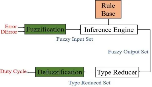
A fuzzy controller typically consists of four parts: Fuzzification, Inference, Rule Base, and Defuzzification, as shown in

Fig. 4.

Fig. 3 The Fuzzy Logic Controller diagram

In this paper, the inputs of the FL controller are the Error and the change of error DError. They are given by the Eqs. (9)

and (10):

 

_{ }



_

1



_

1 P k P k Error k

V k V k

 



  (9)

( ) ( ) ( 1)

DError k Error k Error k (10)

where k, P, and V are the sampling time, the PV panel power and the PV Panel voltage, respectively.

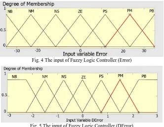
In the fuzzification stage, the digital inputs are converted into seven linguistic variables that are: Positive Big (PB),

Positive Medium (PM), Positive Small (PS), Zero (ZE), Negative Small (NS), Negative Medium (NM), and Negative Big

(NB). Fig. 4 and Fig. 5 present the linguistic variables of the Error and DError.

Fig. 4 The input of Fuzzy Logic Controller (Error)

Fig. 5 The input of Fuzzy Logic Controller (DError)

It is important to understand how the system works to create the rules. In this work, the inference engine based on

(5)

Table 1 Fuzzy Logic rule base

Error DError

PB PB PM PS ZE NS NM PM ZE ZE ZE NB NB NB PS ZE ZE ZE NM NM NM ZE ZE ZE ZE NS NS NM NS NS NS ZE ZE ZE PS NM PM PM PS NS ZE PS NB PM PM PM PB ZE ZE

Based on these rules, the change in the duty cycle is calculated. The output, as presented in Fig. 6, has 7 levels: Positive

Big (PB), Positive Medium (PM), Positive Small (PS), Zero (ZE), Negative Small (NS), Negative Medium (NM), and

Negative Big (NB). In the defuzzification stage, the output is converted to a numerical variable to provide an analog signal.

Thus, the duty cycle of DC/DC Buck Converter is varied to reach the MPP.

Fig. 6 The output of Fuzzy Logic Controller (Duty Cycle)

4.2. Fuzzy logic type 2 (FLT2)

Fuzzy Logic Type 2 (FLT2), noted , models uncertainty better than conventional fuzzy logic. It is characterized by a

three-dimensional membership function u_( , )x y . FLT2 can be expressed by Eq. (11):

( , ) , x x X u j

u x y u x   

 

_{ }

,j_x

 

0,1 ₍₁₁₎

where X, Jx, and ∬ are the primary variable, the primary membership of x and the union of all the Cartesian product elements

on x, respectively.

Each three-dimensional membership function has superior and inferior membership functions represented by classical

fuzzy logic. The interval between the inferior and superior membership functions is called Footprint of Uncertainty (FOU). It is

the new third dimension of the FLT2 which gives more precision, compared to the classical Fuzzy logic [35]. The block

diagram of the FLT2, presented in Fig.7, contains five parts: Fuzzification, Inference Engine, Rule Base, Reducer Type, and

Defuzzification.

(6)

In the fuzzification stage, the two digital inputs (Error and DError) are converted into 3 linguistic variables which are:

Positive (P), Zero (Z), and Negative (N). Each variable has two levels: lower U and higher L. The variables then become (PL,

PU); (ZL, ZU), and (NL, NU). The inputs used in this paper are shown in Fig. 8 and Fig. 9.

Fig. 8 Membership function for Error Fig. 9 Membership function for DError

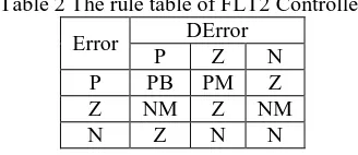
The structure of the rules remains exactly the same in the case of FL algorithm. Table 2 summarizes the rules used in the

employed FLT2 controller.

Table 2 The rule table of FLT2 Controller

Error DError

P Z N

P PB PM Z

Z NM Z NM

N Z N N

The inference engine combines fuzzy rules to perform a transformation from fuzzy sets in the input space to fuzzy sets in

the output space. There are several methods of inference such as the max-min inference method (Mamdami), the max-product

inference method (Larsen) and the AND inference method (Sugeno).

In this paper, the Sugeno method is used. The output of the Inference Engine block is equal to the weighted average of the

output of each fuzzy rule. The FLT2 controller differs from the FL by the output processing module which consists, in this case,

of two blocks: Type Reducer and Defuzzification. For an FLT2 system, each output set of a rule is Type 2. Consequently, the

Type Reducer is used to get a classic set from the Type 2 output sets. The classic set obtained from the Type Reducer is

converted into a well-defined numerical value, in the Defuzzification step, to control the DC/DC Buck Converter.

As numerical value CA of the output, it can be obtained by the Eq. (12):

1 1

(

)

( )

(

)

N

k À k

k

A N

k À k

y u

y

c

x

u

y

 





(12)

where N, y, and uӐ are, respectively, the number of rules, the output, and the membership function.

The simulation results of the two algorithms studied will be presented in the following section. In addition, they will be

compared to the InC Algorithm.

5. Simulation Results

In this part, the simulation results, under MATLAB/Simulink, are presented. The system, shown in Fig. 11, is composed

of six Tesla Solar modules (Solar TS250-P150-60), a DC/DC Buck Converter, MPPT Controller and four series batteries

(7)

Table 3 The specifications of the PV Panel Parameter Value

Pm 255 W

Imp 8.32 A

Vmp 30.6 V

Isc 8.75 A

Vsc 37.6 V

Rsh 529.6538 Ω Rs 0.29192 Ω Module efficiency 15.58%

FL, FLT2, and InC MPPT Algorithms are tested via the MATLAB/Simulink environment in the case of stable and

variable irradiation.

Fig. 10 The global system in Matlab/Simulink

5.1. Uniform irradiation

The simulations of the PV system with the FL, FLT2, and Inc algorithms are done under uniform irradiation (880W/m²)

and fixed temperature (26°C). The voltage and the current of the PV array are used as inputs to calculate the error and the

variation of error that represent the input of the FL an FLT2 controllers as shown in Fig. 11 and Fig. 12. They are designed

following the steps in the previous section.

(8)

Fig. 12 FLT2 algorithm in Matlab/Simulink

Fig. 13 The PV Voltage with InC, FL, and FLT2 MPPT algorithms

Fig. 14 The PV Current with InC, FL, and FLT2 MPPT algorithms

Fig. 15 The PV Power with InC, FL, and FLT2 MPPT algorithms

Fig.13, Fig. 14, and Fig.15 present PV Voltage, PV Current and PV Power, respectively. Fig.15 shows that the power

obtained by InC oscillates between 1265 and 1272W and the MPP is reached at t=0.25s. With FL, the power is equal to 1300W

(9)

remarkable stability. The maximum power is 1335W, which offers better results than those of the FL and InC controllers in

terms of speed and output power.

Fig. 16 shows the Output Voltage of the DC/DC Buck Converter.

Fig. 16 The Output Voltage of Buck Converter with InC, FL, and FLT2 MPPT algorithms

5.2. Non-uniform irradiation

To test the performance of the three algorithms in different climatic conditions, non-uniform irradiation is applied to the

input of the PV array. The irradiation takes 880W/m2 at the beginning of the simulations. After t=3.2 s, it rapidly decreases to

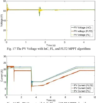
310W/m2 and returns to the initial state. Fig. 17, Fig. 18, and Fig. 19 show the voltage, current, and power generated from the

PV array with the three algorithms (FLT2, FL, InC) in the case of variable irradiation. After the disturbance, the FLT2

controller shows a better performance in term of response time, stability and generated power.

(10)

Fig. 20 shows the variation of the Output Voltage of the Buck Converter in the case of variable irradiation.

Fig. 20 The output voltage of buck converter with InC, FL, and FLT2 MPPT algorithms

6. Experimental Results

In order to verify the real working of the studied MPPT Algorithms, a hardware setup was implemented, as shown in

Fig. 21.

Fig. 21 Experimental setup with the PV array

The setup consists of six Tesla Solar modules (Solar TS250-P150-60), a DC/DC Buck Converter, CompactRio Controller,

National instrument Modules, irradiation sensor (IRRB2 THIES), temperature sensor (LM35) and load. For voltage

measurement, NI 9225 (Analog Input Module, 300Vrms) is connected in parallel with the PV array. NI 9247 (Analog Input

Module, 50 Arms) is connected in series with the PV array to sense the current. All sensed Data is given to the National

Instrument CompactRio NI 9025, an embedded real-time controller. It controls the MOSFET of the DC/DC Buck Converter

using NI 9474. The studied algorithms are programmed and implemented using LabVIEW Software. LabVIEW is a graphical

software from NI for system design, measurement, and control. The choice of this software is based on the ease of

(11)

To read the experimental results, the Front Panel of LabVIEW Software is used. The observed parameters, collected from

the CompactRio are irradiation, temperature, PV current, PV voltage, PV Power and Buck Voltage, as presented in Fig. 22. FL,

FLT2, and InC are tested via LabVIEW environment in the case of stable and variable irradiation. Those experiments were

done on May 2, 2019, on a sunny day. The measured parameters are shown in the figures below.

Fig. 22 LabVIEW Front Panel of the MPPT Algorithms

6.1. Uniform irradiation

The experiment of the PV system with the FL, FLT2, and Inc algorithms are done under uniform irradiation (880W/m²)

and fixed temperature (26°C).

Fig. 23 Experimental results of InC MPPT Algorithm at stable climatic conditions

Fig. 24 Experimental results of FL MPPT Algorithm at stable climatic conditions

(12)

Fig. 23, Fig. 24 and, Fig. 25 present InC, FL and FLT2 experimental results, respectively. Fig. 23 shows that the power

obtained by InC oscillates between 1217. With FL, the power is equal to 1271W. It reaches the MPP and remains stable. By

using an FLT2 controller, the MPP reaches 1335W, which offers better results than those of the FL and InC controllers in terms

of speed and output power.

6.2. Non-uniform irradiation

To test the performance of the three algorithms in different climatic conditions, a variation of the incidence angle of

irradiation was made. The irradiation takes 880W/m2 at the beginning of the simulations. After t=3.2 s, it rapidly decreases to

310W/m2 and returns to the initial state. The variation of the irradiation was obtained by the change of solar incidence angle.

Fig. 26, Fig. 27, and Fig. 28 show the experimental results of InC, FL, and FLT2 MPPT algorithms in the case of variable

irradiation. After the disturbance, the FLT2 controller shows a better performance in term of response time, stability and

generated power.

Fig. 26 Experimental results of InC MPPT Algorithm at variable irradiation

Fig. 27 Experimental results of FL MPPT Algorithm at variable irradiation

Fig. 28 Experimental results of FLT2 MPPT Algorithm at variable irradiation

7. Discussion

From the previous simulations and experimental tests, we can see that the studied MPPT controllers make it possible to

reach the MPP in the case of FL, FLT2, and InC algorithms. In the case of stable and variable irradiation, FLT2 controller is

faster than FL and InC controllers. In addition, the power obtained with FLT2 controller is higher.

The number of rules in the FL controller is very high, which stabilizes the system around the MPP but, at the same time,

makes the controller more complex and increases the calculation time while the FLT2 controller uses a minimized number of

rules with Lower and Upper Standard Deviations to help avoid uncertainties and reduce computation time. Unfortunately,

(13)

The results of this work are presented in table 4. It gives the PV power and the efficiency of the three controllers. The

difference between experimental results and simulations is due to several factors such as measurement errors and losses in the

conversion chain.

Table 4 Simulation and experimental results of InC, FL and FLT2 MPPT algorithms Simulation results Experimental results Techniques PV Power (W) Efficiency (%) PV Power (W) Efficiency (%)

InC 1265-1272 94.22 1217 90.14

FL 1300 96.29 1271 94.14

FLT2 1335 98.81 1288 95.40

8. Conclusions

The objective of this paper is to extract the maximum power of a photovoltaic system using FL, FLT2, and InC MPPT

algorithms.

The proposed system was studied under two different conditions; fix and variable irradiation. MATLAB/Simulink

environment is used for simulation studies and LabVIEW Software for experimental tests. The simulation results and

experimental tests show that the best MPPT technique is FLT2. It shows high performance and gives a good track of MPP with

a minimized response time, it presents high robustness in case of disturbances. InC shows its limit in response time and

stability. In addition, FL algorithm is a robust and powerful technique that does not require exact knowledge of the

photovoltaic system. However, FLT2 is more difficult to use and understand than FL and InC. The difference between

experimental and simulations results is due to several factors such as measurement errors and losses in the conversion chain.

As a perspective, the InC, FL, and FLT2 MPPT Algorithms will be tested in the case of a grid-connected system.

Conflicts of Interest

The authors declare no conflict of interest.

References

[1] Ilyas, M. Ayyub, M. R. Khan, A. Jain, and M. A. Husain, “ Realisation of incremental conductance the MPPT algorithm for a solar photovoltaic system,” International Journal of Ambient Energy, vol. 39, no. 8, pp. 873-884, 2017.

[2] K. P. J. Pradeep, C. C. Mouli, K. S. P. Reddy, and K. N. Raju, “Design and implementation of maximum power point tracking in photovoltaic systems,” International Journal of Engineering Sciences Invention, vol. 4, no. 3, pp. 37-43, March 2015.

[3] H. Bounechba, A. Bouzid, H. Snani, and A. Lashab, “Real-time simulation of MPPT algorithms for PV energy system,” Electrical Power and Energy System, vol. 83, pp. 67-78, December 2016.

[4] K. Rohit, C. Anurag, K. Govind, S. Amritpreet, and Y. Akhlendra, “Modelling/simulation of MPPT techniques for photovoltaic systems using Matlab,” International Journal of Advanced Research in Computer Science and Software Engineering, vol. 7, no. 4, pp. 178-187, April2017.

[5] M. Bachar, A. Naddami, S. Hayani, and A. Fahli, “Design and dimensioning of desalination mobile unit and optimization of electrical energy with MPPT algorithms,” Proc. Americain Institut of Physics, pp. 1-18, December 2018.

[6] M. R. Kumar, S. S. Narayana, and G. Vulasala, “Advanced sliding mode control for solar PV array with fast voltage tracking for MPP algorithm,” International Journal of Ambient Energy, pp. 1-9, 2018.

[7] S. Yaqin, G. Tingkun, D. Yan, Z. Linghan, and T. Jingxuan, “Photovoltaic array maximum power point tracking based on improved perturbation and observation method,” Journal of Physics: Conference Series, vol. 1087, pp. 1-6, 2018. [8] S. Y. Alsadi, “Maximum power point tracking simulation for photovoltaic systems using perturb and observe algorithm,”

International Journal of Web Engineering and Technology, vol. 2, no. 6, pp. 80-85, 2012.

(14)

[10] N. Karami, N. Moubayed, and R. Outbib, “General review and classification of different MPPT techniques,” Renewable and Sustainable Energy Reviews, vol. 68, pp. 1-18, 2017.

[11] M. A. M. Ramli, S. Twaha, K. Ishaque, and Y. A. Al-Turki, “ A review on maximum power point tracking for photovoltaic systems with and without shading conditions,” Renewable and Sustainable Energy Reviews, vol. 67, pp. 144-159, 2017.

[12] C. Larbes, S. M. Aït Cheikh, T. Obeidi, and A. Zerguerras, “Genetic algorithms optimized fuzzy logic control for the maximum power point tracking in a photovoltaic system,” Renewable Energy, vol. 34, no. 10, pp. 2093-2100, 2009. [13] U. Yilmaz, A. Kircay, and S. Borekci, “PV system fuzzy logic MPPT method and PI control as a charge controller,”

Renewable and Sustainable Energy Reviews, vol. 81, pp. 994-1001, 2018.

[14] V. Dabra, K. K. Paliwal, P. Sharma, and N. Kumar, “Optimization of the photovoltaic power system: a comparative study,” Protection and Control of Modern Power Systems, vol. 2, no. 3, pp. 1-11, January 2017.

[15] M. Biglarbegian, W. W. Malek, and J. M. Mendel, “On the stability of interval type-2 TSK fuzzy logic control systems,” IEEE Transactions On Systems, vol. 40, no. 3, pp. 798-818, June 2010.

[16] J. H. Agrawal and M. V. Aware, “Photovoltaic simulator developed in Labview for evaluation of MPPT techniques,” Proc. International Conference on Electrical, Electronics, and Optimization Techniques, March 2016, pp. 1142-1147.

[17] A. El-Leathey, A. Nedelcu, S. Nicolaie, and R.A. Chihaia, “Labview design and simulation of a small scale microgrid,” Series C: Electrical Engineering, vol. 78, no. 1, pp. 235-246, March 2016.

[18] V. Banu, M. Istrate, D. Machidon, and R. Pantelimon, “Study regarding modeling photovoltaic arrays using test data in Matlab/Simulink,” Scientific Bulletin Series C, vol. 77, no. 2, pp. 227-234, 2015.

[19] R. Sridhar, S. Jeevananthan, and P. Vishnuram, “Particle swarm optimization maximum power point tracking approach based on irradiation and temperature measurements for partially shaded photovoltaic system,” International Journal of Ambient Energy, vol. 38, no. 7, 2017.

[20] A. Ayaz and L. Rajaji, “Real-time implementation of the solar inverter with novel MPPT control algorithm for residential application,” Energy and Power Engineering, vol. 5, no. 6, pp. 427-435, August 2013.

[21] S. Kolsi, H. Samet, and M. Ben Amar, “Design analysis of DC-DC converters connected to a photovoltaic generator and controlled by MPPT for optimal energy transfer throught a clear day,” Journal of Power and Energy Engineering, vol. 2, no. 1, pp. 27-34, January 2014.

[22] A. Attou, A. Massoum, and M. Saidi, “Photovoltaic power control using MPPT and boost converter,” Balkan Journal of Electrical & Computer Engineering, vol. 2, no. 1, pp. 23-27, September 2014.

[23] M. Bachar, A. Naddami, S. Hayani, and A. Fahli, “Optimization of PV panel using P&O and incremental conductance algorithms for desalination mobile unit,” Advanced Intelligent Systems Applied to energy, vol. 2, pp. 164-184, January 2019.

[24] R. Faranda and S. Leva, “Energy comparison of MPPT techniques for PV Systems,” WSEAS Transactions on Power Systems, vol. 3, no. 6, pp. 446-455, 2008.

[25] A. Montecucco and A. R. Knox, “Maximum power point tracking converter based on the open-circuit voltage method for thermoelectric generators,” IEEE Transactions on Power Electronics, vol. 30, no. 2, pp. 828-839, March 2014.

[26] A. Dolora, R. Faranda, and S. Leva, “Energy Comparison of Seven MPPT Techniques for PV Systems,” Journal of Electromagnetic Analysis and Applications, vol. 3, pp. 152-162, 2009.

[27] S. Malathy and R. Ramaprabha, “Maximum Power Point Tracking based on look up table approach,” Advanced Materials Research, vol. 768, pp. 124-130, September 2013.

[28] A. Naidu, S. A. Kumar, and G. S. Reddy, “Voltage based P&O algorithm for maximum power point tracking using Labview,” Innovative Systems Design and Engineering, vol. 7, no. 5, pp. 12-16, 2016.

[29] Y. Shi, R. Li, Y. Xue, and H. Li, “High-frequency-link-based grid-tied PV system with small dc-link capacitor and low-frequency ripple-free maximum power point tracking,” IEEE Transactions on Power Electronics, vol. 31, no. 1, pp. 328-339, 2016.

[30] M. Farayola, A. N. Hasan, and A. Ali, “Curve fitting polynomial technique compared to ANFIS technique for maximum power point tracking,” Proc. 8th International Renewable Energy Congress, March 2017.

[31] S. E. Babaa, M. Armstrong, and V. Pickert, “Overview of maximum power point tracking control methods for PV systems,” Journal of Power and Energy Engineering, vol. 2, pp. 59-72, 2014.

[32] M. E. Başoğlu and B. Çakir, “Design and implementation of DC-DC converter with Inc-Cond algorithm,” International Journal of Electrical Energetic Electronic and Communication Engineering, vol. 9, no. 1, pp. 45-48, January 2015. [33] W. M. Lin, C. M. Hong, and C. H. Chen, “Neural-network-based MPPT control of a stand-alone hybrid power generation

(15)

[34] M. Kermadi and E. M. Berkouk, “Artificial intelligence-based maximum power point tracking controllers for photovoltaic systems: comparative study,” Renewable and Sustainable Energy Reviews, vol. 69, pp. 369-386, 2017.

[35] M. S. Fadali, S. Jafarzadeh, and A. Nadeh, “Fuzzy TSK approximation using Type-2 fuzzy logic systems and its application to modeling a photovoltaic array,” Proc. American Control Conference, pp. 6454-6459, July 2010.