Multi-Task Learning for Straggler Avoiding Predictive Job
Scheduling
Neeraja J. Yadwadkar [email protected]
Division of Computer Science University of California
Berkeley, CA 94720-1776, USA
Bharath Hariharan [email protected]
Division of Computer Science University of California
Berkeley, CA 94720-1776, USA
Joseph E. Gonzalez [email protected]
Division of Computer Science University of California
Berkeley, CA 94720-1776, USA
Randy Katz [email protected]
Division of Computer Science University of California
Berkeley, CA 94720-1776, USA
Editor:Urun Dogan, Marius Kloft, Francesco Orabona, and Tatiana Tommasi
Abstract
Parallel processing frameworks (Dean and Ghemawat, 2004) accelerate jobs by breaking them into tasks that execute in parallel. However, slow running orstraggler tasks can run up to 8 times slower than the median task on a production cluster (Ananthanarayanan et al., 2013), leading to delayed job completion and inefficient use of resources. Existing straggler mitigation techniques wait to detect stragglers and then relaunch them, delaying straggler detection and wasting resources. We built Wrangler (Yadwadkar et al., 2014), a system that predicts when stragglers are going to occur and makes scheduling decisions to avoid such situations. To capture node and workload variability, Wrangler built separate models for every node and workload, requiring the time-consuming collection of substantial training data. In this paper, we propose multi-task learning formulations that share infor-mation between the various models, allowing us to use less training data and bring training time down from 4 hours to 40 minutes. Unlike naive multi-task learning formulations, our formulations capture the shared structure in our data, improving generalization perfor-mance on limited data. Finally, we extend these formulations using group sparsity inducing norms to automatically discover the similarities between tasks and improve interpretability.
1. Introduction
con-sequence of such a parallel execution model is that the slow-running tasks, commonly called
stragglers, potentially delay overall job completion. In a recent study, Ananthanarayanan et al. (2013) show that straggler tasks are on an average 6 to 8 times slower than the median task of the corresponding job, despite existing mitigation techniques. Suri and Vassilvitskii (2011) describe the intensity of straggler problem as the “curse of the last reducer”, causing the last 1% of the computation to take much longer to finish execution. Mitigating strag-glers thus remains an important problem. In this paper, our focus is on machine learning approaches for predicting and avoiding these stragglers.
Existing approaches to straggler mitigation, whether reactive or proactive, fall short in multiple ways. Commonly used reactive approaches such as speculative execution (Dean and Ghemawat, 2004), act after the tasks have already slowed down. Proactive approaches that launch redundant copies of a task in a hope that at least one of them will finish in a timely manner (Ananthanarayanan et al., 2013), waste resources. It is hard to, a priori, identify which factors, and configurations lead to stragglers, motivating a data driven ma-chine learning approach to straggler prediction. Bortnikov et al. (2012) explored predictive models for predicting slowdown for tasks. But they learn a single model for a cluster of nodes, ignoring the variability caused due to the heterogeneity across nodes and across jobs from different workloads. Moreover, they built models but did not show if these models could indeed improve job completion times, which is what matters ultimately. Gupta et al. (2013) explored learning based job scheduling by matching node capabilities to job require-ments. However, their approach is not designed to deal with stragglers effectively because it does not model the time-varying state of the nodes (for instance, how busy they are). Moreover, the effectiveness of these methods in reducing job-completion times in real world clusters hasn’t been shown. To this end, we built Wrangler (Yadwadkar et al., 2014), a system that builds predictive models of straggler behavior and incorporates this model in the scheduler, improving the 99th percentile job completion time by up to 61% as
com-pared to speculative execution for real world production level workloads1 from Facebook
and Cloudera’s customers.
Proactive model based approaches including Wrangler, have previously treated each workload and even compute node as a separate straggler estimation task with independent models. The decision to model each workload and node independently is motivated by the observation that the resource contention patterns that cause stragglers can vary from node to node and workload to workload. For a detailed analysis about causes of stragglers across nodes and workloads, see Section 4.2.2. of Wrangler, Yadwadkar et al. (2014). To address such heterogeneity in the nodes and changing workload patterns, training sepa-rate models for each workload being run on each node, is considered necessary. However, such independent models pose two critical challenges: (1) each new node and workload re-quires new training data which can take hours to collect, delaying the application of model based scheduling, and (2) clusters with many nodes may only have limited data for a given workload on each node leading to lower quality models.
These shortcomings can be addressed if each classifier is able to leverage information gleaned at other nodes and from other workloads. For instance, when there is not enough
data at a node for a workload, we can gain from the data collected at that node while it was executing other workloads, or from other nodes running the same workload. Such information sharing falls in the ambit of multi-task learning (MTL), where the learner is embedded in an environment of related tasks, and the learner’s aim is to leverage similarities between the tasks to improve performance of all tasks.
In this paper, we propose an MTL formulation for learning predictors that are more accurate and generalize better than existing straggler predicting models. Basic MTL for-mulations often assume only limited correlation structure between learning tasks. However, our application has an additional overlapping group structure: models built on the same node for different workloads can be grouped together, as can be the models correspond-ing to the same workload runncorrespond-ing on different nodes. We propose a new formulation that leverages this overlapping group structure, and show that doing so significantly reduces the number of parameters and improves generalization to tasks with very little data.
In applications such as ours, high accuracy is not the only objective: we also want to be able to gain some insight into what is causing these stragglers. Such insight can aid in debugging root causes of stragglers and system performance degradation. Automatically learned classifiers can be opaque and hard to interpret. To this end, we propose group sparsity inducing mixed-norm regularization on top of our basic MTL formulation to auto-matically reveal the group structure that exists in the data, and hopefully provide insights into how straggler behavior is related across nodes and workloads. We also explore sparsity-inducing formulations based on feature selection that attempt to reveal the characteristics of straggler behavior.
For our experimental evaluation, we use a collection of real-world workloads from Face-book and Cloudera’s customers. We evaluate not only the prediction accuracy but also the improvement in job completion times, which is the metric that directly impacts the end user. We show that our formulation to predict stragglers allows us to reduce job completion times by up to 59% over the previous state-of-the-art learning base system, Wrangler (Yadwadkar et al. (2014)). This large reduction arises from a 7 point increase in prediction accuracy. Further, we can get equal or better accuracy than Wrangler (Yadwadkar et al. (2014)) using a sixth of the training data, thus bringing the training time down from 4 hours to about 40 minutes. We also provide empirical evidence that compared to naive MTL formulations, our formulation indeed generalizes to new tasks, i.e, it is significantly better at predicting straggler behavior for nodes for which we have not collected enough data.
Finally, while our initial motivation and experimental validation focus on the straggler avoidance problem, our learning formulations are general and can be applied to other sys-tems that train node or workload dependent classifiers (Gupta et al., 2013; Delimitrou and Kozyrakis, 2014). For instance, ThroughputScheduler (Gupta et al., 2013) uses such clas-sifiers to allot resources to tasks, and can benefit from such multitask reasoning. We leave these extensions to future work.
To summarize, our key contributions are:
2. A mixed-norm group sparsity inducing formulation, that automatically detects group structure (Section 4.3) facilitating interpretability.
3. An efficient optimization technique based on a reduction to the standard SVM (Cortes and Vapnik (1995)) formulation (Section 4.2).
4. A comprehensive evaluation as part of a complete system for predicting and avoiding stragglers in real world production cluster traces (Section 5). We show that, compared to existing approaches, our formulations
(a) avoid stragglers better with 7% improved prediction accuracy, improving job completion times significantly with up to 57.8% improvement in the 99th
per-centile, and reducing net resource usage by up to 40%, and
(b) can work even with a sixth of the training data and thus a much shorter training period, reducing the training data collection time significantly from 4 hours to 40 minutes.
In what follows, we first give some background on stragglers in Section 2. We then describe Wrangler and discuss its shortcomings in Section 3. In Section 4, we describe our multi-task learning formulations. In Section 5, we empirically evaluate our formulations on real world production level traces from Facebook and Cloudera’s customers. We end with a discussion of related work.
2. Background and Motivation
The growing popularity of Internet-based applications, in addition to reduced costs of stor-age media, has resulted in generation of data at an unprecedented scale. Analytics on such huge datasets has become a driving factor for business. Parallel processing on commodity clusters has emerged as the de-facto way of dealing with the scale and complexity of such data-intensive applications. Dean and Ghemawat (2004) originally proposed the MapRe-duce framework at Google to process enormous amounts of data. MapReMapRe-duce is highly scalable to large clusters of inexpensive commodity computers. Hadoop (White, 2009), an open source implementation of MapReduce, has been widely adopted by industry over the last decade.
A data intensive application is submitted to a cluster of commodity computers as a MapReducejob. To accelerate completion, MapReduce divides a job into multipletasks. A cluster scheduler assigns these to machines (nodes), where they are executed in parallel. A job finishes when all its tasks have finished execution. A key benefit of such frameworks is that they automatically handle failures (which are more likely to occur on a cluster of commodity computers) without needing extra efforts from the programmer. Two basic modes of failures are the failure of a node and the failure of a task. If a node crashes, MapReduce re-runs all the tasks it was executing on a different node. If a task fails, MapReduce automatically re-launches it.
tasks have finished execution, such slow-running tasks, called stragglers, extend the job’s completion time. This, in turn, leads to increased user costs.
Stragglers abound in the real world. According to Ananthanarayanan et al. (2013), if stragglers did not exist in real-world production clusters, the average job completion times would have been improved by 47%, 29% and 36% in the Facebook, Bing and Yahoo traces respectively. We observed that 22-28% of the total tasks are stragglers in a replay2 of
Facebook and Cloudera’s customers’ Hadoop production cluster traces. Thus, stragglers are a major hurdle in achieving faster job completions.
It is challenging to deal with stragglers (Dean and Ghemawat, 2004; Zaharia et al., 2008; Ananthanarayanan et al., 2010). Dean and Ghemawat (2004) mentioned that stragglers could arise due to various reasons, such as competition for resources, problematic hardware, and mis-configurations. Ananthanarayanan et al. (2010) report that consistently slow nodes are rarely the reason behind stragglers; the majority are caused by transient node behavior. The reason is simple: cluster schedulers assign multiple tasks, belonging to the same or different jobs, to be executed simultaneously on a node. Depending on the node’s characteristics and current load, as well as the characteristics of the workloads, these jobs may result in counterproductive resource contention patterns. Moreover, this gives rise to dynamically changing task execution environments, causing large variations in task execution times. We cannot simply look at the initial configuration of the node and decide if it will cause stragglers. We must track the continuously changing state of the node (its memory usage, cpu usage etc.) and use that to predict straggler behavior.
Above and beyond this temporal variability is the variability across nodes and workloads. If the scheduler assigns memory hungry tasks on a memory-constrained node, stragglers could occur due to contention for memory. While for another node that has slower disk, straggler behavior will primarily depend on how many I/O-intensive tasks are being run. To predict straggler behavior, we need to consider both the current state of each node and tailor the decision to the node type (its resource capabilities) and particular kind of tasks being executed (their resource requirements). In our experiments, we find that models that do not take this into account do about 6-7% worse than models that do (see Table 5 in Section 5.3).
Due to these difficulties in understanding the causes behind stragglers, and the chal-lenges involved in predicting stragglers, initial attempts at mitigating stragglers have been
reactive (Dean and Ghemawat, 2004; Zaharia et al., 2008; Ananthanarayanan et al., 2010). Dean and Ghemawat (2004) suggestedspeculative execution as a mitigation mechanism for stragglers. This is a reactive scheme that is dominantly used on production clusters includ-ing those at Facebook and Microsoft Binclud-ing (Ananthanarayanan et al., 2014). It operates in two steps: (1) wait-and-speculate if a task is executing slower than other tasks of the same job, and (2) replicate or spawn multiple redundant copies of such tasks hoping a copy will reach completion before the original. As soon as one of the copies or the original task finishes execution, the rest are killed.
The benefits of Speculative execution, in terms of improved job completion times at the cost of resources consumed, are unclear. Due to the wait-and-speculate step, this scheme is inefficient in time, leading to a delay before speculation begins. Also, due to the second
Trace % of speculatively executed tasks that were killed
Facebook 2009 (FB2009) 77.9%
Facebook 2010 (FB2010) 88.6%
Cloudera’s Customer b (CC b) 74.4%
Cloudera’s Customer e (CC e) 48.8%
Table 1: Majority of the speculatively executed tasks eventually get killed since the original task finishes execution before them.
step that replicates tasks, such mechanisms lead to increased resource consumption without necessarily gaining performance benefits. Moreover, we observed that the original task, that was marked as a straggler in the wait-and-speculate step, often finishes execution before any of the redundant copies launched in the second step. Thus, a significant number of such redundant copies end up getting killed, resulting in wastage of resources and perhaps additional unnecessary contention. Table 1 shows that about 48% to 88% of the specu-latively executed copies were killed in our replay of Facebook and Cloudera’s customers’ production cluster traces. LATE (Zaharia et al., 2008) improves over speculative execution using a notion of progress scores, but still results in resource wastage due to replication.
Since reactive mechanisms fall short of efficiently mitigating stragglers, some proactive approaches have been proposed. Dolly (Ananthanarayanan et al., 2013) is a cloning mech-anism that avoids the wait-and-speculate phase of speculative execution and immediately launches redundant copies of tasks belonging to small jobs. However, being replication-based, it also incurs resource overhead.
Machine learning has shown promise in dealing with the challenges of estimating task completion times and predicting stragglers in parallel processing environments (Bortnikov et al., 2012; Gupta et al., 2013). We built Wrangler (Yadwadkar et al., 2014) (see Section 3), a system that learns to predict nodes that might create stragglers and uses these predictions as hints to the scheduler so as to avoid creating stragglers by rejecting bad placement decisions. Thus, being proactive, Wrangler is time efficient. Also, by smarter scheduling, we avoid replication of straggler tasks. Thus, Wrangler is also efficient in terms of reducing the resources consumed. Wrangler was the first complete system that demonstrated the utility of learning methods in reducing job-completion times in real world clusters.
In the following sections, we review Wrangler, describe its architecture, discuss its limi-tations and avenues for improvements. Then in Section 4, we present our multi-task learning based approach that improves upon Wrangler by resolving its limitations.
3. Wrangler
using these models, for whether the task will become a straggler. It then uses this prediction to modify the scheduling decisions if straggler behavior is predicted. Section 3.4 provides a brief explanation of the predictive scheduler.
3.1 Features and labels
To predict whether scheduling a task at a particular node will lead to straggler behav-ior, Wrangler uses the resource usage counters at the node. Dean and Ghemawat (2004) mentioned that stragglers could arise due to various reasons such as competition for CPU, memory, local disk, network bandwidth. Zaharia et al. (2008) further suggest that strag-glers could be caused due to faulty hardware and misconfiguration. Ananthanarayanan et al. (2010) report that the dynamically changing resource contention patterns on an underlying node could give rise to stragglers. Based on these findings, we collected the performance counters for CPU, memory, disk, network, and other operating system level counters de-scribing the degree of concurrency before launching a task on a node. The counters we collected span multiple broad categories as follows:
1. CPU utilization: CPU idle time, system and user time and speed of the CPU, etc.
2. Network utilization: Number of bytes sent and received, statistics of remote read and write, statistics of RPCs, etc.
3. Disk utilization: The local read and write statistics from the datanodes, amount of free space, etc.
4. Memory utilization: Amount of virtual, physical memory available, amount of buffer space, cache space, shared memory space available, etc.
5. System-level features: Number of threads in different states (waiting, running, termi-nated, blocked, etc.), memory statistics at the system level.
In total, we collect 107 distinct features characterizing the state of the machine. See Sec-tion 5.1 for details of our dataset.
Features: Multiple tasks from jobs of each workload may be run on each node. There-fore to simplify notation, we index the execution of a particular task by iand define Sn,l
as the set of tasks corresponding to workload lexecuted on node n. Before executing task
i∈Sn,l corresponding to workload l on node nwe collect the resource usage counters
de-scribed above on node n to form the feature vector xi ∈R107. For each feature described
above we subtract the minimum across the entire dataset and rescale so that it lies between 0 and 1 for the entire dataset.
Labels: After running task iwe measure the normalized task duration nd(i) which is the ratio of task execution time to the amount of work done (bytes read/written) by task
i. From the normalized duration, we determine whether a task has straggled using the following definition:
Definition 1 A task i of a job J is called a straggler if
nd(i)> β×median
wherend(i)is the normalized duration of taskicomputed as the ratio of task execution time to the amount of work done (bytes read/written) by task i.
In this paper, as in Wrangler, we setβ to 1.3. Given the definition of a straggler, for task
iwe define yi ∈ {0,1} as a binary label indicating whether the corresponding taskiended up being a straggler relative to other tasks in the same job.
3.2 Prediction Task
While the resource usage counters do track the time-varying state of the node, they do not model the variability across nodes, or the properties of the particular task we are executing. To deal with the variability of nodes, Wrangler builds a separate predictor for each node.
Modeling the variability across tasks is harder since it would require understanding the code that the task is executing. Instead, Wrangler uses the notion of “workloads”, which we define next. Companies such as Facebook, Google, use compute clusters for various computational purposes. The specific pattern of execution of jobs on these clusters is called aworkload. These workloads are specified using various statistics, such as submission times of multiple jobs, number of their constituent tasks along with their input data sizes, shuffle sizes, and output sizes. Wrangler assumes that all tasks in a particular workload have similar properties in terms of resource requirements etc., and it captures the variability across workloads by building separate predictors for each workload. Thus Wrangler builds separate predictors for each node and for every workload.
Putting it all together, we can state the binary classification problem for predicting straggler tasks more formally as follows. A datapoint in our setting corresponds to a task
iof job J from a particular workloadl that is executed on a nodenin our cluster. Before running task i we collect the features xi which characterize the state of node n. After
running task i we then measure the normalized duration and determine whether the task straggled with respect to other tasks of job J (see Definition 1). Our goal is to learn a function:
fn,l :x−→y,
for each noden and workload l that maps the current characteristics x∈Rd of that node
(e.g., current CPU utilization) to the binary variable y ∈ {0,1} indicating whether that task will straggle (i.e., run longer than β times the median runtime).
3.3 Training
For any workload l, Wrangler first collects data and ground truth labels for training and validation. In particular, for every task ilaunched on node n, Wrangler records both the resource usage counters xi and the label yi which indicates if the task straggles or not. Since there is a separate predictor for each node and workload, Wrangler produces separate datasets for each node and workload. LetSn,l be the set of tasks of jobs corresponding to
workloadl, executed on noden. Thus, we record the dataset for noden, workloadl as:
Dn,l ={(xi, yi) :i∈Sn,l}.
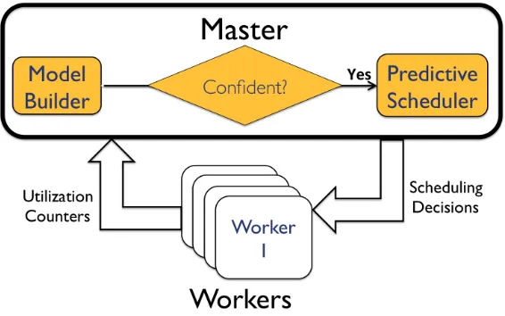
Figure 1: Architecture of Wrangler.
then trained on these datasets. Stragglers, by definition are fewer than the non-straggler tasks. Therefore for training, Wrangler statistically oversampled the class of stragglers to avoid the skew in the strengths of the two classes. This gets the two classes represented equally.
After this initial training phase, the classifiers are frozen, and the trained classifiers are incorporated into the job scheduler as described above. They are then tested on the next Ttest= 10 hours by measuring the impact of these classifiers on job completion times.
Further details about the train and test splits are in Section 5.
3.4 Model-aware scheduling
Job scheduling in Hadoop is handled by a master, which controls the workers. The master assigns tasks to the worker nodes. The assignments depend upon the number of available slots as well as data-locality. Wrangler modifies this scheduler to incorporate its predictions. Before launching a task i of a job coming from a workload l, on a node n, the scheduler collects the node’s resource usage counters xi and runs the classifier fn,l. If the classifier predicts that the task will be a straggler with high enough “confidence” (Wrangler uses SVMs with scaling by Platt (1999) to produce a confidence), the scheduler does not assign the task to that node. It is later assigned to a node that is not predicted to create a straggler. See Yadwadkar et al. (2014) for details on the algorithm and implementation.
3.5 Shortcomings of Wrangler and avenues for improvements
production clusters with tens of thousands of nodes, it might be a long time before a node collects enough data to train a classifier. (In Table 5 we show that the prediction accuracy of Wrangler rapidly degrades as the amount of training data is reduced). In some cases, workloads may only be run a few times in total, limiting the ability of systems like Wrangler to make meaningful predictions.
Alternatively, large clusters with locality aware scheduling can lead to poor sample coverage. Recall that, in our case, each task of a workload executed on a node amounts to a training data point. The placement of input data on nodes in a cluster is managed by the underlying distributed file system (Ghemawat et al., 2003). To achieve locality for faster reading of input data, sophisticated locality-aware schedulers (Zaharia et al., 2008, 2010) try to assign tasks to nodes already having the appropriate data. Based on the popularity of the data, number of tasks assigned to a node could vary. Hence, we may not get uniform number of training data points, i.e., tasks executed, across all the nodes in a cluster. There could be other reasons behind skewed assignment of tasks to nodes (Kwon et al., 2012): even when every map task has the same amount of data, a task may take longer depending on the code path it takes based on the data it processes. Hence, the node slots will be busy due to such long running tasks. This could lead to some nodes executing fewer tasks than others.
These observations suggest that our modeling framework needs to be robust to limited and potentially skewed data. Thus, there is a need for straggler prediction models (1) that can be trained using minimum available data, and (2) that generalize to unseen nodes or workloads. In the following section, we describe our multi-task learning based approach with these goals for avoiding stragglers. We evaluate it using real world production level traces from Facebook and Cloudera’s customers, and compare the gains with Wrangler.
4. Multi-task learning for straggler avoidance
As described in the previous section, Wrangler builds separate models for each workload and for every node. Thus, every {node, workload} tuple is a separate learning problem. However, learning problems corresponding to different workloads executed on the same node clearly have something in common, as do learning tasks corresponding to different nodes executing the same workload. We want to use this shared structure between the learning problems to reduce data collection time.
We turn to multi-task learning to leverage this shared structure. In the terminology of multi-task learning, each {node, workload} pair forms a separate learning-task3 and these
learning problems have a shared structure between them. However, unlike typical MTL formulations, our learning-tasks are not simply correlated with each other; they share a specific structure, clustering along node- or workload-dependent axes. In what follows, we first describe a general MTL formulation that can capture such learning-task grouping. We then detail how we apply this formulation to our application of straggler avoidance.
4.1 Partitioning tasks into groups
Suppose there areT learning tasks, with the training set for the t-th learning-task denoted by Dt ={(xit, yit) :i= 1, . . . , kt}, with xit∈Rd. We begin with the formulation proposed
by Evgeniou and Pontil (2004). Evgeniou, et al. proposed a basic hierarchical regression formulation with the linear model,wt, for learning-task t as:
wt=w0+vt (2)
The intuition here is that w0 captures properties common to all learning-tasks, while vt
captures how the individual learning-tasks deviate from w0.
We then frame learning in the context of empirical loss minimization. Given the vari-ability in node behavior and the need for robust predictions we adopt the hinge-loss and applyl2 regularization to both the basew0 and learning-task specific weights vt:
min w0,vt,b
λ0kw0k2+ λ1
T T X
t=1
kvtk2+ T X
t=1 kt
X
i=1
LHinge
yit,(w0+vt)Txit+b
(3)
whereLHinge(yit, sit) = max(0,1−yitsit) is the hinge loss.
In the above formulation, all learning-tasks are treated equivalently. However, as dis-cussed above, in our application some learning-tasks naturally cluster together. Suppose that the learning-tasks cluster intoGnon-overlappinggroups, with thet-th learning-task be-longing to theg(t)-th group. Note that while we derive our formulations for non-overlapping groups, which is true in our application, the modification for overlapping groups is trivial. Using the same intuition as Equation 2, we can write the classifier wt as:
wt=w0+vt+wg(t) (4)
In general, there may be more than one way of dividing our learning-tasks into groups. In our application, one may split learning-tasks into groups based on workload or based on nodes. We call one particular way of dividing learning-tasks into groups a partition. The
p-th partition has Gp groups, and the learning-tasktbelongs to the gp(t) group under this
partition. Now, we also have a separate set of weight vectors for each partition p, and the weight vector of theg-th group of thep-th partition is denoted bywp,g. Then, we can write
the classifier wt as:
wt=w0+vt+ P X
p=1
wp,gp(t) (5)
Finally, note thatw0 and vtcan also be seen as weight vectors corresponding to trivial
partitions: w0corresponds to the partition where all learning-tasks belong to a single group,
and vt corresponds to the partition where each learning-task is its own group. Thus, we
can includew0 andvt in our partitions and write Equation 5 as:
wt= P X
p=1
wp,gp(t) (6)
Intuitively, at test time, we get the classifier for the t-th learning-task by summing weight vectors corresponding to each group to which tbelongs.
As in Equation 3, the learning problem involves minimizing the sum of l2 regularizers on each of the weight vectors and the hinge loss:
min wp,g,b
P X p=1 Gp X g=1
λp,gkwp,gk2+ T X t=1 kt X i=1 LHinge yit,
P X
p=1
wp,gp(t)
T
xit+b
(7)
Here, the regularizer coefficient λp,g = λp#(p,g)
T , where #(p, g) denotes the number of
learning-tasks assigned to theg-th group of thep-th partitioning. The scaling factorλp#(p,g)
T
interpolates smoothly betweenλ0, when all learning-tasks belong to a single group, and λ1T ,
when each learning-task is its own group. Loweringλp for a particular partition will reduce the penalty on the weights of thep-th partition and thus cause the model to rely more on thep-th partitioning. For the base partitionp= 0, settingλp = 0 would thus favor as much
parameter sharing as feasible.
4.2 Reduction to a standard SVM
One advantage of the formulation we use is that it can be reduced to a standard SVM (Cortes and Vapnik, 1995), allowing the usage of off-the-shelf SVM solvers. Below, we show how this reduction can be achieved. Given λ, for every group g of every partitionp, define:
˜
wp,g= r
λp,g
λ wp,g (8)
Now concatenate these vectors into one large weight vector ˜w:
˜
w= [ ˜wT1,1, . . . ,w˜p,gT , . . . ,w˜TP,GP]T (9) Then, it can be seen that λkw˜k2 =PP
p=1 PGp
g=1λp,gkwp,gk2. Thus, with this change of
variables, the regularizer in our optimization problem resembles a standard SVM. Next, we transform the data pointsxit intoφ(xit) such that we can replace the scoring function with
˜ wTφ(x
it). This transformation is as follows. Again, define:
φp,g(xit) =δgp(t),g
s λ
Here,δgp(t),g is a kronecker delta, which is 1 ifgp(t) =g(i.e. , if the learning-task tbelongs
to group g in the p-th partitioning) and 0 otherwise. Our feature transformation is then the concatenation of all these vectors:
φ(x) = [φ1,1(x)T, . . . , φp,g(x)T, . . . , φP,GP(x)
T]T (11)
It is easy to see that:
˜
wTφ(xit) =
P X
p=1
wp,gp(t)
T
xit (12)
Intuitively, ˜wconcatenates all our parameters with their appropriate scalings into one long weight vector, with one block for every group of every partitioning. φ(xit) transforms a data
point into an equally long feature vector, by placing scaled copies ofxit in the appropriate
blocks and zeros everywhere else.
With these transformations, we can now write our learning problem as :
min
˜
w,b λkw˜k 2+
T X
t=1 kt
X
i=1
LHinge(yit,w˜Tφ(xit) +b) (13)
which corresponds to a standard SVM. In practice, we use this transformation and change of variables, both at train time and at test time.
4.3 Automatically selecting groups or partitions
In many real world applications including our own, good classification accuracy is not an end in itself. Model interpretability is of critical importance. A large powerful classifier working on tons of features may do a very good job of classification, but will not provide any insight to an engineer trying to identify the root causes of a problem. It will also be difficult to debug such a classifier if and when it fails. In the absence of sufficient training data, large models may also overfit. Thus, interpretability and simplicity of the model are important goals. In the context of the formulation above, this means that we want to keep only a minimal set of groups/partitions while maintaining high classification accuracy.
We can use mixed l1 and l2 norms to induce a sparse selection of groups or
parti-tions (Bach et al., 2011). Briefly, suppose we are given a long weight vector wdivided into
M blocks, with them-th block denoted bywm. Then the squared mixedl1 and l2 norm is:
Ω(w) =
M X
m=1
kwmk2 !2
(14)
This can be considered as anl1 norm on a vector with elements kwmk2. When Ω(·) is used
as a regularizer, the l1 norm will force some elements of this vector to be set to 0, which in
turn would force the corresponding block of weights wm to be set to 0. It thus encourages
entire blocks of the weight vector to be set to 0, a sparsity pattern that is often called “group sparsity”.
1. We can put all the weight vectors corresponding to a single partition in the same block. Then, the regularizer becomes:
Ωps( ˜w) =
P X
p=1 kw˜pk2
2
(15)
where ˜wp = [ ˜wTp,1, . . . ,w˜Tp,Gp]
T concatenates all weight vectors corresponding to the
p-th partition. This regularizer will thus tend to kill entire partitions. In other words, it will uncover notions of grouping, or learning-task similarity, that are the most important.
2. We can put the weight vector of each group of each partition in separate blocks. Then the regularizer becomes:
Ωgs( ˜w) =
P X
p=1 G X
g=1
kw˜p,gk2
2
(16)
This regularizer will tend to select a small set of groups which are needed to get a good performance.
4.4 Automatically selecting features
Mixed norms can also be used to select a sparse set of feature blocks that are most useful for classification. This is again useful for interpretability. In our application, features are resource counters at a node. Some of these features are related to memory, others to cpu usage, etc. If our model is able to predict straggler behavior solely on the basis of memory usage counters, for instance, then it might indicate that the cluster or the workload is memory constrained.
In our multi-task setting, such feature selection can also interact with the different groups and partitions of learning-tasks. Suppose each feature vectorxis made up of blocks corresponding to different kinds of features, denoted byx(1),x(2), . . .x(B). We can similarly
divide each weight vector ˜wp,g into blocks denoted by ˜w(1)p,g, ˜w(2)p,g and so on. Then we have
two alternatives.
1. One can concatenate corresponding feature blocks from all the weight vectors to get ˜
w(1), . . . ,w˜(B). Then a mixed l
1 and l2 regularizer using these weight blocks can be
written as:
Ωf s1( ˜w) = B X
b=1
kw˜(b)k2 !2
(17)
2. An alternative would be to let each group vector choose its own sparse set of feature blocks. This can be achieved with the following regularizer:
Ωf s2( ˜w) = X
p,g B X
b=1
kw˜p,g(b)k2 !2
(18)
4.5 Kernelizing the formulation
We have till now described our formulation in primal space. However, kernelizing this formulation is simple. First, note that if we use a simple squared l2 regularizer, then
our formulation is equivalent to a standard SVM in a transformed feature space. This transformed feature space corresponds to a new kernel:
Knew(xit,xju) = hφ(xit), φ(xju)i
= X
p,g
hφp,g(xit), φp,g(xju)i
= X
p,g
δgp(t),gδgp(u),g λ
λp,gK(xit,xjt) (19)
Thus, the transformed kernel corresponds to the linear combination of a set of kernels, one for each group. Each group kernel is zero unless both data points belong to the group, in which case it equals a scaled version of the kernel in the original feature space.
When using the mixed-norm regularizers, the derivation is a bit more involved. We first note that (Aflalo et al., 2011):
M X
m=1
kwmk2 !2
= min
0≤η≤1,kηk1≤1 M X
m=1
kwmk22 ηm
(20)
Using this transformation leads to the following primal objective:
min w,b,0≤η≤1,kηk1≤1
M X
m=1
kwmk22 ηm +
X
i,t
L(xit, yit,w) (21)
whereL(xit, yit,w) is the hinge loss. This corresponds to a 1-norm multiple kernel learning
formulation (Kloft et al., 2011) where each block of feature weights corresponds to a separate kernel. We refer the reader to Kloft et al. (2011) for a description of the dual of this formulation.
We note that these kernelized versions are very similar to the ones derived in (Widmer et al., 2010; Blanchard et al., 2011). However, the group and partition structure and the application domain are unique to ours.
4.6 Application to straggler avoidance
We apply this formulation to straggler avoidance as follows. Suppose there areN nodes and
FB2009
Node 1 Node 2 Node 3
FB2010 CC_e
v
1⌃
⌃
⌃
⌃
⌃
⌃
⌃
⌃
⌃
v
2v
3v
4v
5v
6v
7v
8v
9w
0w
f b09w
node1w
1=
w
0+
w
node1+
w
f b09+
v
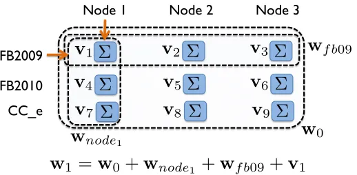
1Figure 2: In our context of straggler avoidance, the learning-tasks naturally cluster into various groups in multiple partitions. When a particular learning- task, for example, node 1 and workload FB2009 (v1), has
limited training data available, we learn its weight vector, w1, by adding the weight vectors of groups it
belongs to from different partitions.
1. A single group consisting of all nodes and workloads. This gives us the single weight vectorw0.
2. One group for each node, consisting of all L learning-tasks belonging to that node. This gives us one weight vector for each node wn, n = 1, . . . , N, that captures the
heterogeneity of nodes.
3. One group for each workload, consisting of all N learning-tasks belonging to that workload. This gives us one weight vector for each workload wl, l = 1, . . . , L, that captures peculiarities of particular workloads.
4. Each {node, workload}tuple as its own group. Since there are N ×L such pairs, we get N ×L weight vectors, which we denote as vt, following the notation considered
in Evgeniou and Pontil (2004).
Thus, if we use all four partitions, the weight vector wt for a given workload lt and a
given nodent is:
wt=w0+wnt +wlt +vt (22)
Figure 2 shows an example. The learning problem for the FB20094 workload running on
node 1 belongs to one group from each of the four partitions mentioned above: (1) the global partition, denoted by the weight vector, w0, (2) the group corresponding to node 1 from
the node-wise partition, denoted by the weight vectorwnode1, (3) the group corresponding
to the FB2009 workload from the workload-wise partition, denoted by the weight vector
wf b09, and (4) the group containing just this individual learning problem, denoted by the
weight vector v1. Thus, we can learn the weight vectorw1 as:
w1 =w0+wnode1+wf b09+v1 (23)
The corresponding training problem is then:
min
w,b λ0kw0k 2+ ν
N N X
n=1
kwnk2+ ω L
L X
l=1
kwlk2+ τ T
T X
t=1 kvtk2
+ T X t=1 kt X i=1 LHinge
yit,(w0+wnt+wlt +vt)
Tx it+b
(24)
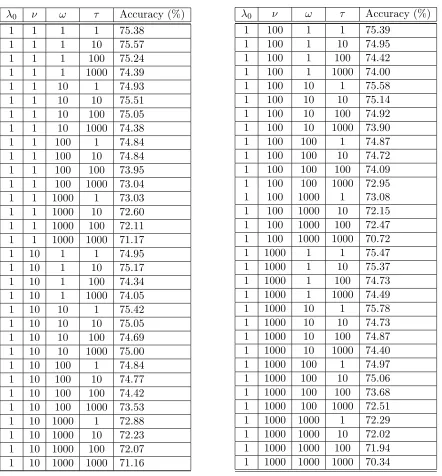
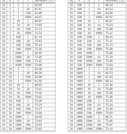
where λ0, ν, ω, τ are hyperparameters. We ran an initial grid search on a validation set to fix these hyperparameters and found that prediction accuracy was not very sensitive to these settings: several settings gave very close to optimal results. We used λ0 = ν = ω = τ = 1, which was one of the highest performing settings, for all our experiments. Appendix A provides the details of this grid search experiment along with the sensitivity of these hyperparameters to a set of values. As described in Section 4.2, we work in a transformed space in which the above problem reduces to a standard SVM. In this space the weight vector is
˜
w= [ ˜wT0,w˜n1T , . . . ,w˜nTN,w˜l1T, . . . ,w˜TlL,v˜Tt1, . . . ,v˜TtT]T (25) This decomposition will change depending on which partitions we use.
As described in the previous section, we can also use mixed l1 and l2 norms to auto-matically select groups or partitions. To select partitions, we combine all the node-related weight vectors ˜wn1, . . . ,w˜nN into one long vector ˜wN, all workload vectors ˜wl1, . . . ,w˜lL
into ˜wL and all ˜v1, . . . ,v˜T into ˜vT. We then solve the following optimization:
min ˜
w,b (kw˜0k2+kw˜Nk2+kw˜Lk2+kv˜Tk2) 2
+CX
i,t
LHinge yit,w˜Tφ(xit) +b
(26)
This model will learn which notion of grouping is most important. For instance if ˜wL
is set to 0, then we might conclude that straggler behaviour doesn’t depend that much on the particular workload being executed.
To select individual groups, we solve the optimization problem:
min ˜
w,b,ξ≥0 kw˜0k2+ N X
n=1
kw˜nk2+ L X
l=1
kw˜lk2+ T X
t=1 kv˜tk2
!2
+CX
i,t
LHinge yit,w˜Tφ(xit) +b
(27)
This formulation can set some individual node or workload models to 0. This would mean that straggler behavior on some nodes or workloads can be predicted by generic models, but others require more node-specific or workload-specific reasoning.
in Section 3.1: counters based on cpu, those based on network, those based on disk, those based on memory, and other system-level counters. Then each ˜wn, ˜wl and ˜vtgets similarly
split up. As described before, we can either let each model choose its own set of features using this regularizer:
Ω( ˜w) = (kw˜mem
0 k2+kw˜disk0 k2+kw˜cpu0 k2+kw˜network0 k2+kw˜system0 k2+
+PN
n=1[kw˜nmemk2+kw˜diskn k2+kw˜cpun k2+kw˜networkn k2+kw˜systemn k2]
+PL
l=1[kw˜meml k2+kw˜diskl k2+kw˜cpul k2+kw˜networkl k2+kw˜systeml k2]
+PT
t=1[kv˜memt k2+kv˜tdiskk2+kv˜tcpuk2+kv˜networkt k2+kv˜tsystemk2])2 (28)
or choose a single set of features globally using this regularizer:
Ω( ˜w) =kw˜memk2+kw˜cpuk2+kw˜diskk2+kw˜networkk2+kw˜systemk2 2
(29)
where ˜wmem concatenates all memory related weights from all models,
˜
wmem = [ ˜wmemT0 ,w˜n1memT, . . . ,w˜nmemTN ,w˜l1memT, . . . ,w˜memTlL ]T (30) ˜
wcpu, ˜wdisk etc. are defined similarly.
4.7 Exploring the relationships between the weight vectors
Before getting into the experiments, we can get some insights on what our formulation will learn by looking at the KKT conditions. Equation 24 can equivalently be written as:
min
w,b,ξλ0kw0k 2+ ν
N N X
n=1
kwnk2+ ω L
L X
l=1 kwlk2
+τ
T T X
t=1
kvtk2+ T X t=1 kt X i=1
ξit (31)
s.t. yit
(w0+wnt +wlt +vt)
Tx it+b
≥1−ξit ∀i, t ξit≥0 ∀i, t
The Lagrangian of the formulation in Equation 31 is:
L(w, b,α,γ) =λ0kw0k2+ ν N
N X
n=1
kwnk2+ ω L
L X
l=1 kwlk2
+τ
T T X
t=1
kvtk2+ T X t=1 kt X i=1 ξit−
T X t=1 kt X i=1
γitξit (32)
+ T X t=1 kt X i=1
Taking derivatives w.r.t the primal variables and setting to 0 gives us relationships between
w0,vt,wn and wl:
λ0w∗0 = τ T
X
t
vt∗ (33)
νw∗n= τ
T /N X
t:nt=n
vt∗ (34)
ωw∗l = τ
T /L X
t:lt=l
vt∗ (35)
λ0w∗0 = ν
N X
n
wn∗ (36)
λ0w∗0 = ω L
X
l
wl∗ (37)
Evgeniou and Pontil (2004) also obtain Equation 33 in their formulation, but the other relationships are specific to ours. These relationships imply that these variables shouldn’t be considered independent. wn,wl and w0 are scaled means of the vt’s of the group they
capture.
4.8 Generalizing to unseen nodes and workloads
Consider what happens when we remove the partition corresponding to individual {node, workload} tuples, i.e., vt, from our formulations. We now do not have any parameters
specific to a node-workload combination, but can still capture both node- and workload-dependent properties of the learning problem. Such formulations are thus similar to fac-torized models where the node and workload dependent factors are grouped into separate blocks. We end up with only (N+L)dparameters, whereas a formulation like that of (Ev-geniou and Pontil, 2004; Ev(Ev-geniou et al., 2005; Jacob et al., 2009) will still have N Ld
parameters (here d is the input dimensionality). Thus, we can reduce the number of pa-rameters while still capturing the essential properties of the learning problems.
In addition, since we no longer have a separate weight vector for each{node, workload}
tuple, we can generalize to node-workload pairs that are completely unseen at train time: the classifier for such an unseen combination t will simply be w0 +wnt +wlt. We thus
explicitly use knowledge gleaned from prior workloads run on this node (throughwnt) and
other nodes running this workload (throughwlt). This is especially useful in our application
where there may be a large number of nodes and workloads. In such cases, collecting data for each node-workload pair will be time consuming, and generalizing to unseen combinations will be a significant advantage.
In most of our experiments, therefore, we remove the partition corresponding to indi-vidual {node, workload}tuples. We explicitly evaluate how well we generalize by doing so in Section 5.4.
5. Empirical Evaluation
Trace #Machines Length Date #Jobs
FB2009 600 6 month 2009 1129193
FB2010 3000 1.5 months 2010 1169184
CC b 300 9 days 2011 22974
CC e 100 9 days 2011 10790
Total ≈4000 ≈8.5 months - 2332141
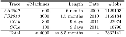
Table 2: Dataset. FB: Facebook,CC: Cloudera Customer.
sufficient data and also when sufficient data is not available, and second, improvement in overall job completion times, and third, reduction in resources consumed.
5.1 Datasets
The set of real-world workloads considered in this paper are collected from the production compute clusters at Facebook and Cloudera’s customers, which we denote as F B2009,
F B2010, CC b and CC e. Table 2 provides details about these workloads in terms of the number of machines in the actual clusters, the length and date of data capture, total number of jobs in those workloads. Chen, et al., explain the data in further details in (Chen et al., 2012). Together, the dataset consists of traces from over about 4000 machines captured over almost eight months. For faithfully replaying these real-world production traces on our 20 node EC2 cluster, we used a statistical workload replay tool, SWIM (Chen et al., 2011) that synthesizes a workload with representative job submission rates and patterns, shuffle/input data size and output/shuffle data ratios (see Chen et al. (2011) for details of replay methodology). SWIM scales the workload to the number of nodes in the experimental cluster.
For each workload, we need data with ground-truth labels for training and validating our models. We collect this data by running tasks from the workload as described above and recording the resource usage counters xi at a node at the time a task i is launched, and the ground truth label yi by checking if it ends up becoming a straggler. Then we divide this dataset temporally into a training set and a validation set. In other words, the first few tasks that were executed form the train set and the rest of the tasks form the validation set. In the experiments below, we vary the percentage of data that is used for training, and compute the prediction accuracy on the validation set. We train our final model using two-thirds of this dataset and proceed to evaluate it on our ultimate metric, i.e., job completion times.
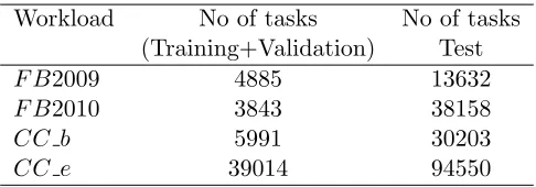
To measure job completion times, we then incorporate the trained models into the job scheduler (as in Wrangler). We then run the replay for the workload again, but with a fresh set of tasks. These fresh set of tasks form our test set, and this test set is only used to measure job completion times. Table 3 shows the sizes of the datasets.
Each data point is represented by a 107 dimensional feature vector comprising the node’s resource usage counters at the time of launching a task on it. We optimize all our formulations using Liblinear (Fan et al., 2008) for thel2 regularized variants and using the
Workload No of tasks No of tasks (Training+Validation) Test
F B2009 4885 13632
F B2010 3843 38158
CC b 5991 30203
CC e 39014 94550
Table 3: Number of tasks we use for each workload in the train+val and test sets.
Below, we describe (1) how we use different MTL formulations and prediction accuracy achieved by these formulations, (2) how we learn a classifier for previously unseen node and/or workload and the prediction accuracy it achieves, (3) the improvement in overall job completion times achieved by our formulation and Wrangler over speculative execution, and (4) reduction in resources consumed using our formulation compared to Wrangler.
5.2 Variants of proposed formulation
We consider several variants of the general formulation described in Section 4. Using a simple squared l2 regularizer, we first considerw0,wnand wl, individually:
• f0: In this formulation, we consider only the global partition in which all learning problems belong to a single group. This corresponds to removing vt, wn and wl.
This formulation thus learns a single global weight vector, w0, for all the nodes and
all the workloads.
• fn: Here we consider only the partition based on nodes. This corresponds to only learning awn, that is, one model for each node. This model learns to predict stragglers
based on a node’s resource usage counters across different workloads, but it cannot capture any properties that are specific to a particular workload.
• fl: Here we consider only the partition based on workloads. This means we only learn
wl, i.e., a workload dependent model across nodes executing a particular workload.
This model learns to predict stragglers based on the resource usage pattern caused due to a workload across nodes, but ignores the characteristics of a specific node.
The above three formulations either discard the node information, the workload infor-mation, or both. We now consider multi-task variants that capture both, node and workload properties:
• f0,t: This is the formulation proposed by Evgeniou and Pontil (2004), and corresponds to using the global partition where all learning-tasks belong to one group, and the partition where each learning-task is its own group. This learnsw0 andvt. Note that
this formulation still has to learn on the order of N Lddifferent parameters, and has to collect enough data to learn a separate weight vector for each {node, workload}
combination.
• f0,n,l: We remove the partition corresponding to individual {node, workload} tuples,
removing vt entirely and only learning w0,wl and wn. As described in Section 4.8,
this formulation reduces the total number of parameters to (N +L)d and can also generalize to unseen{node, workload} tuples.
For all these formulations, the hyperparameters λ0, ν, ω and τ were set to 1 wherever applicable. We found this setting to be close to optimal in our initial cross-validation experiments (see Appendix A).
In addition to these, we also consider sparsity-inducing formulations for automatically selecting partitions or groups or blocks of features, as explained in Sections 4.3, 4.4, and 4.6.
• fps : We use the global, node-based and workload-based formulations thus removing
vtentirely as inf0,n,land use mixedl1 andl2norms to automatically select the useful
partitions from among these. This model will learn the notion of grouping that is most important. To select partitions, we combine all the node-related weight vectors
˜
wn1, . . . ,w˜nN into one long vector ˜wN and all workload vectors into ˜wL as shown
below:
˜
w= [ ˜wT
0,w˜Tn1, . . . ,w˜nTN
| {z }
˜
wT N
,w˜T
l1, . . . ,w˜TlL
| {z }
˜
wT L
]T (38)
Thus our weight vector ˜wis split up into blocks corresponding to node, workload and global models.
• fgs : This is the formulation where we use mixed l1 and l2 norms to automatically select groups within a partition. Again, we only consider the global, node-based and workload-based formulations. This formulation can set individual node or workload models to zero, unlike fps, that can set a complete partition, i.e. in our case, a combined model of all the nodes or all the workloads to zero. This would mean that predicting straggler behavior on some nodes or workloads does not need reasoning that is specific to those nodes or workloads; instead a generic model would work.
Finally, we also try the following two mixed norms formulations for feature selection. As before, both these formulations remove the partition corresponding to individual{node, workload}tuples, i.e., remove vt.
• ff s1 : As explained in Equation 28, we divide our features into five categories
corre-sponding to cpu, memory, disk, network and other system-level counters. Then each weight vector gets similarly split up into these categories. This formulation learns which categories of features are more important for some nodes or workloads than others.
• ff s2 : This formulation, as given in Equation 29, selects a category of features across
5.3 Prediction accuracy
In this section, we evaluate the formulations described in the previous section for their straggler prediction accuracy. In the following subsection 5.3.1, we evaluate formulations that use l2 regularizers, viz., f0, fn, fl, f0,n,l, f0,t, and f0,t,l. Then, in Section 5.3.2, we
evaluate the mixed norm formulations (a) that automatically selects partitions, fps, (b)
that automatically selects groups, fgs, and then the formulations (c) ff s1, and (d) ff s2
that can automatically select features. We list our formulations with a brief description in Table 4.
5.3.1 Formulations with l2 regularizers
We aim at learning to predict stragglers using as small amount of data as feasible, as this means shorter data capture time. Note that stragglers are fewer than non-stragglers, so we oversample from the stragglers’ class to represent the two classes equally in both, the training and validation sets5. Table 5 shows the percentage accuracy of predicting stragglers
with varying amount of training data. We observe that:
• With very small amounts of data, all MTL variants outperform Wrangler. In fact, all of f0 tof0,t,l need only one sixth of the training data to achieve the same or better accuracy.
• It is important to capture both node- and workload-dependent aspects of the problem:
f0,n,l, f0,t andf0,t,l consistently outperformf0, fn and fl.
• f0,t and f0,t,l perform up to 7 percentage points better than Wrangler with the same
amount of training data, withf0,n,l not far behind.
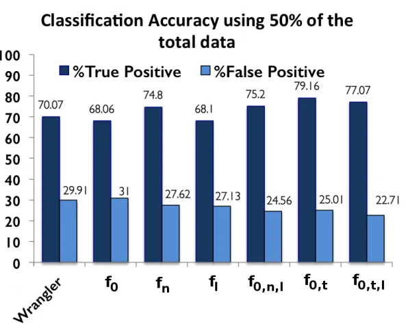
For a better visualization, Figure 3 shows the comparison of prediction accuracy of these formulations, in terms of percentage true positives and percentage false positives when 50% of total data is available.
Next, we evaluate and discuss the sparsity-inducing formulations,fps (Equation 26),fgs
(Equation 27), ff s1 (Equation 28), andff s2 (Equation 29).
5.3.2 Formulations with mixed l1 and l2 norms
Automatically selecting partitions or groups: In this Section, we evaluate fps and fgs. Table 6 shows the prediction accuracy of these formulations compared tof0,fn,fl and f0,n,l. fps andfgs show comparable prediction accuracy tof0,n,l. We also found interesting
sparsity patterns in the learnt weight vectors.
• fps : Recall that fps attempts to set the weights of entire partitions to 0. In our case we have a global partition, a node-based partition and a workload-based partition. We observed that only ˜w0 is zero in the resulting weight vector learned. This means that
given node-specific and workload-specific factors, the global factors that are common across all the nodes and workloads do not contribute to the prediction. In other words, similar accuracy could be achieved without using ˜w0. However, both
node-and workload-dependent weights are necessary.
Formulation Description
f0 uses a single, global weight vector
fn uses only node-specific weights
fl uses only workload-specific weights
f0,n,l uses global, node- and workload-specific weights
f0,t uses global weights and weights specific to{node, workload} tuples
f0,t,l uses global and workload-specific weights and weights specific to {node, workload}tuples fps selects partitions automatically
fgs selects groups automatically
ff s1 selects feature-blocks automatically for individual groups ff s2 selects feature-blocks automatically across all the groups
Table 4: Brief description of all our formulations.
%Training Wrangler
f0 fn fl f0,n,l f0,t f0,t,l
Data Yadwadkar et al. (2014)
1 Insufficient data 66.9 63.5 66.5 65.5 63.7 66.2
2 Insufficient Data 67.1 63.3 67.7 67.5 64.3 67.7
5 Insufficient Data 67.5 68.1 69.1 69.8 69.6 69.1
10 63.9 67.8 70.9 69.4 72.3 73.1 72.9
20 67.2 68.0 72.6 70.1 72.9 74.7 74.8
30 68.5 68.5 73.2 70.3 74.1 75.9 75.8
40 69.7 68.2 73.9 70.5 74.3 76.4 76.4
50 70.1 68.5 74.1 70.4 75.3 77.1 77.2
Table 5: Prediction accuracies (in %) of various MTL formulations for straggler prediction with varying amount of training data. See Section 5.3.1 for details.
• fgs : In fgs, we encourage individual nodes-specific or individual workloads-specific weight vectors separately to be set to zero. We observed that some of the nodes’ weight vectors and some of the workload-specific weight vectors were zero, indicating that in some cases we do not need node or workload specific reasoning. (One can use the learnt sparsity pattern and attempt to correlate it with some node and workload characteristics; however we have not explored this in this paper.)
We also note that our mixed-norm formulations automatically learn a grouping that achieves comparable accuracy with lesser total number of groups, and thus fewer parameters.
Figure 3: Classification accuracy of various MTL formulations as compared to Wrangler using 50% of the total data. This plot shows the percentage of true positives and the percentage of false positives in each of the cases. These quantities are computed as: % True Positive = (fraction of stragglers predicted correctly as stragglers)×100, and % False Positive = (fraction of non-stragglers predicted incorrectly to be stragglers)
×100.
Formulation Straggler Prediction Accuracy
f0 68.5
fn 74.1
fl 70.4
f0,n,l 75.3
fps 74.4
fgs 73.8
Table 6: Straggler prediction accuracies (in %) using the four mixed-norm formulationsfpsandfgscompared with formulations that usel2 regularizers. Note that fps andfgs perform with comparable accuracy with
f0,n,l, however, use lesser number of groups and parameters, resulting in simpler models.
Table 7 shows the percentage prediction accuracies of these formulations on our test set. Note that these formulations show comparable prediction accuracy. Next, we discuss the impact offf s1 and ff s2 on understanding the straggler behavior.
Formulation Straggler Prediction Accuracy (in %)
ff s1 74.9 ff s2 74.9
Table 7: Straggler prediction accuracies (in %) usingff s1 andff s2 that encourage sparsity across bocks of
features.
FB2009 FB2010 CC b CC e
f0,n,l f0,t f0,n,l f0,t f0,n,l f0,t f0,n,l f0,t
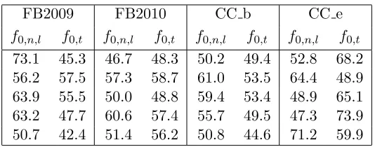
73.1 45.3 46.7 48.3 50.2 49.4 52.8 68.2 56.2 57.5 57.3 58.7 61.0 53.5 64.4 48.9 63.9 55.5 50.0 48.8 59.4 53.4 48.9 65.1 63.2 47.7 60.6 57.4 55.7 49.5 47.3 73.9 50.7 42.4 51.4 56.2 50.8 44.6 71.2 59.9
Table 8: Straggler Prediction accuracies (in %) off0,n,landf0,ton test data from an unseen node-workload pair. See Section 5.4 for details.
This reinforces our belief that the causes of stragglers vary quite a bit from node to node or workload to workload.
• ff s2: This formulation considers these feature categories across the various nodes and
workloads and provides a way of knowing if there are certain dominating factors caus-ing stragglers in a cluster. However, we observed that none of the feature categories had zero weights in the weight vector learned for our dataset. Again, this means that there is no single, easily discoverable reason for straggler behavior, and provides evidence to the claim made by Ananthanarayanan et al. (2013, 2014) that the causes behind stragglers are hard to figure out.
5.4 Prediction accuracy for a {node, workload} tuple with insufficient data
One of our goals in this work is to reduce the amount of training data required to get a straggler prediction model up and running. When a new workload begins to execute on a node, we want to learn a model as quickly as possible. Recall that (Section 5.3) with enough training data available we found that f0,n,l, f0,t and f0,t,l seem to perform similarly, with f0,n,l performing slightly worse. However, as mentioned in Section 4.8, formulation f0,n,l
has fewer parameters and, because it has no weight vector specific to a particular {node, workload}tuple, can generalize to new{node, workload} tuples unseen at train time. This is in contrast to f0,t which has to fall back on w0 in such a situation, and thus may not
generalize as well. In this section, we see if this is indeed true.
We trained classifiers based on f0,n,l and f0,t leaving out 95% of the data of one
node-workload pair every time. We then test the models on the left-out data. Table 8 shows the percentage classification accuracy from 20 such runs. We note the following:
• For 13 out of 20 classification experiments,f0,n,lperforms better thanf0,t. For 10 out of these 13 cases, the difference in performance is more than 5 percentage points.
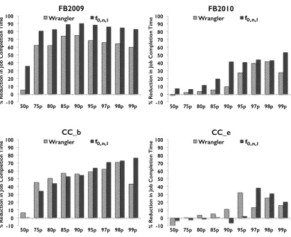
Figure 4: Improvement in the overall job completion times achieved byf0,n,land Wrangler over speculative execution.
• f0,n,l sometimes performs worse, but in only 3 of these cases is it significantly worse (worse by more than 5 percentage points). All 3 of these instances are in case of the
CC e workload. In general, for this workload, we also notice a huge variance in the numbers obtained across multiple nodes. See Yadwadkar et al. (2014), for a discussion of some of the issues in this workload.
This shows thatf0,n,lworks better in real-world settings where one cannot expect enough
data for all node-workload pairs. Therefore, we evaluate f0,n,l in our next experiment (Section 5.5) to see if it improves job completion times.
5.5 Improvement in overall job completion time
We now evaluate our formulation,f0,n,l, using the second metric, improvement in the overall
job completion times over speculative execution. We compare these improvements to that achieved by Wrangler (Figure 4). Improvement at the 99th percentile is a strong
Workload % Reduction in total task-seconds (MTL withf0,n,l) (Wrangler)
FB-2009 73.33 55.09
FB-2010 8.9 24.77
CC b 64.12 40.15
CC e 13.04 8.24
Table 9: Resource utilization withf0,n,l and with Wrangler over speculative execution, in terms of total task execution times (in seconds) across all the jobs. f0,n,l reduces resources consumed over Wrangler for
F B2009,CC bandCC e.
improves over Wrangler, reflecting the improvements in prediction accuracy. At the 99th
percentile, we improve Wrangler’s job completion times by 57.8%,35.8%,58.9% and 5.7% forF B2009, F B2010, CC bandCC e respectively. Note that Wrangler is already a strong baseline. Hence, the improvement in job completion times on top of the improvement achieved by Wrangler is significant.
5.6 Reduction in resources consumed
When a job is launched on a cluster, it will be broken into small tasks and these tasks will be run in a distributed fashion. Thus, to calculate the resources used, we can sum the resources used by all the tasks. As in Yadwadkar et al. (2014), we use the time taken by each task as a measure of the resources used by the task. Note that, because these tasks will likely be executing in parallel, the total time taken by the tasks will be much larger than the time taken for the whole job to finish, which is what job completion time measures (shown in Figure 4). Ideally, straggler prediction will prevent tasks from becoming stragglers. Fewer stragglers means fewer tasks that need to be replicated by straggler mitigation mechanisms (like speculative execution) and thus lower resource consumption. Thus, improved straggler prediction should also reduce the total task-seconds i.e., resources consumed.
Table 9 compares the percentage reduction in resources consumed in terms of total task-seconds achieved by f0,n,l and Wrangler over speculative execution. We see that the
improved predictions off0,n,lreduce resource consumption significantly more than Wrangler
for 3 out of 4 workloads, thus supporting our intuitions. In particular, for F B2009 and
CC b, f0,n,l reduces Wrangler’s resource consumption by about 40%, while for CC e the
reduction is about 5%.
6. Related Work on Multi-task Learning
The idea that multiple learning problems might be related and can gain from each other dates back to Thrun (1996) and Caruana (1993). They pointed out that humans do not learn a new task from scratch but instead reuse knowledge gleaned from other learning tasks. This notion was formalized by, among others, Baxter (2000) and Ando and Zhang (2005), who quantified this gain. Much of this early work relied on neural networks as a means of learning these shared representations. However, contemporary work has also focused on SVMs and kernel machines.
task-specific component. In later work, Evgeniou et al. (2005) propose an MTL framework that uses a general quadratic form as a regularizer. They show that if the tasks can be grouped into clusters, they can use a regularizer that encourages all the weight vectors of the group to be closer to each other. Jacob et al. (2009) extend this formulation when the group structure is not known a priori. Xue et al. (2007) infer the group structure using a Bayesian approach. The approach of Widmer et al. (2010) is similar to ours and groups tasks into “meta-tasks”, and tries to automatically figure out the meta-tasks required to get good performance. The formulation we propose is also designed to handle group structure, but allows us to dispense with task-specific classifiers entirely, reducing the number of parameters drastically. This allows us to handle tasks that have very little training data by transferring parameters learnt on other tasks. Our formulation shares this property with that of Blanchard et al. (2011), and indeed our basic formulation can be written down in the kernel-based framework they describe for learning to generalize onto a completely unseen task. Other ways of controlling parameters include learning a distance metric (Parameswaran and Weinberger, 2010), and using low rank regularizers (Pong et al., 2010).
Our setting is an example of multilinear multitask learning where each learning problem is indexed by two indices: the node and the workload. Previous work on this subfield of multitask learning has typically used low-rank regularizers on the weight matrix represented as tensors (Romera-Paredes et al., 2013; Wimalawarne et al., 2014). It is also possible to define a similarity between tasks based on how many indices they share (Signoretto et al., 2014). Our formulation captures some of the same intuitions, but has the added advantage of simplicity and ease of implementation.
Using mixed norms for inducing sparsity has a rich history. Donoho (2006) showed that minimizing thel1 norm recovers sparse solutions when solving linear systems. When used
as a regularizer, the l1 norm learns sparse models, where most weights are 0. The most
well known of such sparse formulations is the lasso (Tibshirani, 1996), which uses the l1
norm to select features in regression. Yuan and Lin (2006) extend the lasso to group lasso, where they use a mixed l1 and l2 norm to select a sparse set of groups of features. Bach
(2008) study the theoretical properties of group lasso. Since these initial papers, mixed norms have found use in a variety of applications. For instance , Quattoni et al. (2008) use a mixed l∞ and l1 norm for feature selection. Such mixed norms also show up in the
literature on kernel learning, where they are used to select a sparse set of kernels (Varma and Ray, 2007; Kloft et al., 2011) or a sparse set of groups of kernels (Aflalo et al., 2011). Bach et al. (2011) provides an accessible review of mixed norms and their optimization, and we direct the interested reader to that article for more details.
7. Conclusion