Estimating Diffusion Networks: Recovery Conditions,
Sample Complexity & Soft-thresholding Algorithm
Manuel Gomez-Rodriguez† [email protected]
MPI for Software Systems
Paul-Ehrlich-Strasse, 67663 Kaiserslautern Germany
Le Song [email protected]
College of Computing
Georgia Institute of Technology Atlanta, GA 30332, USA
Hadi Daneshmand [email protected]
Computer Science Department Universit¨atstrasse 6, 8092 Z¨urich Switzerland
Bernhard Sch¨olkopf [email protected]
MPI for Intelligent Systems
Spemannstrasse 38, 72076 T¨ubingen Germany
Editor:Edo Airoldi
Abstract
Information spreads across social and technological networks, but often the network struc-tures are hidden from us and we only observe the traces left by the diffusion processes, called cascades. Can we recover the hidden network structures from these observed cas-cades? What kind of cascades and how many cascades do we need? Are there some network structures which are more difficult than others to recover? Can we design efficient inference algorithms with provable guarantees?
Despite the increasing availability of cascade data and methods for inferring networks from these data, a thorough theoretical understanding of the above questions remains largely unexplored in the literature. In this paper, we investigate the network structure inference problem for a general family of continuous-time diffusion models using an `1
-regularized likelihood maximization framework. We show that, as long as the cascade sampling process satisfies a natural incoherence condition, our framework can recover the correct network structure with high probability if we observeO(d3logN) cascades, where d is the maximum number of parents of a node and N is the total number of nodes. Moreover, we develop a simple and efficient soft-thresholding network inference algorithm
. These authors contributed equally to this work.
. † This work was done while Manuel Gomez-Rodriguez was still affiliated with the MPI for Intelligent Systems, Spemannstr. 38, 72076 Tuebingen, Germany
which demonstrate the match between our theoretical prediction and empirical results. In practice, this new algorithm also outperforms other alternatives in terms of the accuracy of recovering hidden diffusion networks.
1. Introduction
Diffusion of information, behaviors, diseases, or irrepresentabilitymore generally,contagions
can be naturally modeled as a stochastic process that occur over the edges of an underlying network (Rogers, 1995). In this scenario, we often observe the temporal traces that the diffusion generates, calledcascades, but the edges of the network that gave rise to the diffu-sion remain unobservable (Adar and Adamic, 2005). For example, blogs or media sites often publish a new piece of information without explicitly citing their sources. Marketers may note when a social media user decides to adopt a new behavior but cannot tell which neighbor in the social network influenced them to do so. Epidemiologist observe when a person gets sick but usually cannot tell who infected her. In all these cases, given a set of cascades and a diffusion model, the network inference problem consists of inferring the edges (and model parameters) of the unobserved underlying network (Gomez-Rodriguez, 2013).
The network inference problem has attracted significant attention in recent years (Saito et al., 2009; Gomez-Rodriguez et al., 2010, 2011, 2013b, 2014; Snowsill et al., 2011; Du et al., 2012a, 2013; Zhou et al., 2013), since it is essential to reconstruct and predict the paths over which information can spread, and to maximize sales of a product or stop in-fections. Most previous work has focused on developing network inference algorithms and evaluating their performance experimentally on different synthetic and real networks, and a rigorous theoretical analysis of the problem has been missing. However, such analysis is of outstanding interest since it would enable us to answer many fundamental open questions. For example, which conditions are sufficient to guarantee that we can recover a network given a large number of cascades? If these conditions are satisfied, how many cascades are sufficient to infer the network with high probability? Until recently, there has been only two pieces of work along this direction (Netrapalli and Sanghavi, 2012; Abrahao et al., 2013), which leverage less realistic diffusion models. Moreover, none of them is able to identify a recovery condition relating the interaction between the network structure and the cascade sampling process, which we make precise in our paper.
1.1 Overview of results
an `1-regularized maximum likelihood estimator andO(d3logN) cascades, whereN is the number of nodes in the network and dis the maximum number of parents of a node, with the probability of success approaching 1 in a rate exponential in the number of cascades. Importantly, if this condition also holds for the finite sample case, then the guarantee can be improved to O(d2logN) cascades. Beyond theoretical results, we also propose a new, efficient and simple proximal gradient algorithm to solve the `1-regularized maximum like-lihood estimation. The algorithm is especially well-suited for our problem since it is highly scalable and naturally finds sparse estimators, as desired, by using soft-thresholding. Us-ing this algorithm, we perform various experiments illustratUs-ing the consequences of our theoretical results and demonstrating that it typically outperforms other state-of-the-art algorithms.
1.2 Related work
Netrapalli and Sanghavi (2012) propose a maximum likelihood network inference method for a variation of the discrete-time independent cascade model (Kempe et al., 2003) and show that, for general networks satisfying a correlation decay, the estimator recovers the network structure givenO(d2logN) cascades, and the probability of success is approaching 1 in a rate exponential in the number of cascades. The rate they obtained is on a par with our results. However, their discrete diffusion model is less realistic in practice, and the correlation decay condition implies that, on average, each node can only infect one single node per cascade. Instead, we use a general continuous-time diffusion model (Gomez-Rodriguez et al., 2011), which has been extensively validated in real diffusion data and extended in various ways by different authors (Wang et al., 2012; Du et al., 2012a,b).
Abrahao et al. (2013) propose a simple network inference method, First-Edge, for a slightly different continuous-time independent cascade model (Gomez-Rodriguez et al., 2010), and show that, for general networks, if the cascade sources are chosen uniformly at random, the algorithm needs O(N dlogN) cascades to recover the network structure and the probability of success is approaching 1 in a rate polynomial in the number of cas-cades. Additionally, they study trees and bounded-degree networks and show that, if the cascade sources are chosen uniformly at random, the error decreases polynomially as long asO(logN) and Ω(d9log2dlogN) cascades are recorded respectively. In our work, we show that, for general networks satisfying a natural irrepresentability condition, our method out-performs the First-Edge algorithm and the algorithm for bounded-degree networks in terms of rate and sample complexity.
Gripon and Rabbat (2013) propose a network inference method for unordered cascades, in which nodes that are infected together in the same cascade are connected by a path containing exactly the nodes in the trace, and give necessary and sufficient conditions for network inference. However, they consider a restrictive scenario in which cascades are all three nodes long.
2. Continuous-Time Diffusion Model
Figure 1: The diffusion network structure (left) is unknown and we only observe cascades, which areN-dimensional vectors recording the times when nodes get infected by contagions that spread (right). Cascade 1 is (ta, tb, tc,∞,∞,∞), whereta< tc< tb, and cascade 2 is (∞, tb,∞, td, te, tf), where tb < td < te < tf. Each cascade contains a source node (dark red), drawn from a source distributionP(s), as well as infected (light red) and uninfected (white) nodes, and it provides information on black and dark gray edges but does not on light gray edges.
in contrast to previous discrete-time models which associate each edge with a fixed infection probability (Kempe et al., 2003). Moreover, it also differs from discrete-time models in the sense that events in a cascade are not generated iteratively in rounds, but event timings are sampled directly from the transmission functions in the continuous-time model.
2.1 Cascade generative process
Given a directed contact network, G = (V,E) with N nodes, the process begins with an infected source node, s, initially adopting certain contagion (idea, meme or product) at time zero, which we draw from a source distribution P(s). The contagion is transmitted from the source along her out-going edges to her direct neighbors. Each transmission through an edge entails arandom transmission time, τ, drawn from an associated pairwise transmission likelihood f(τ;αji). We assume transmission times are independent, possibly distributed differently across edges, and, in some cases, can be arbitrarily large, τ → ∞. Then, the infected neighbors transmit the contagion to their respective neighbors, and the process continues. We assume that an infected node remains infected for the entire diffusion process. Thus, if a node i is infected by multiple neighbors, only the neighbor that first infects node i will be the true parent. As a result, although the contact network can be an arbitrary directed network, each contagion induces a Directed Acyclic Graph (DAG). Figure 1 illustrates the process and Table 1 gives several examples of well-known parametric transmission likelihoods (Gomez-Rodriguez et al., 2011, 2013a, 2014).
2.2 Cascade data
Observations from the model are recorded as a set Cn of cascades {t1, . . . ,tn}. Each cascadetc is anN-dimensional vectortc:= (tc1, . . . , tcN) recording when nodes are infected,
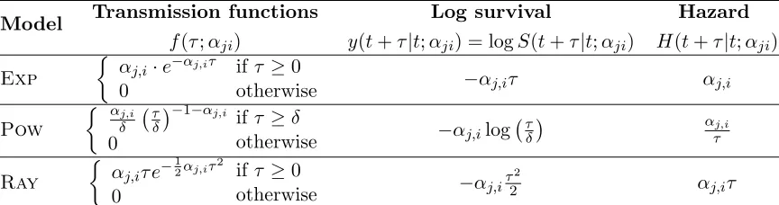
Model Transmission functions Log survival Hazard
f(τ;αji) y(t+τ|t;αji) = logS(t+τ|t;αji) H(t+τ|t;αji)
Exp
αj,i·e−αj,iτ
0
ifτ ≥0
otherwise −αj,iτ αj,i
Pow
αj,i δ
τ δ
−1−αj,i
0
ifτ ≥δ
otherwise −αj,ilog
τ δ
αj,i
τ
Ray
αj,iτ e− 1 2αj,iτ2
0
ifτ ≥0
otherwise −αj,i
τ2
2 αj,iτ
Table 1: Pairwise transmission models
cascade. We assume Tc = T for all cascades; the results generalize trivially. Contagions
often propagate simultaneously (Myers and Leskovec, 2012; Prakash et al., 2012) over the same network but we assume each contagion to propagate independently of each other. Finally, we also assume that all activated nodes except the first one are activated by network diffusion, i.e., by previously activated nodes, ignoring external influences (Myers et al., 2012). Refer to Figure 1 for an example.
2.3 Likelihood of a cascade
Gomez-Rodriguez et al. (2011) showed that the likelihood of a cascadetunder the continuous-time independent cascade model is
f(t;A) = Y
ti≤T
Y
tm>T
S(T|ti;αim)×
Y
k:tk<ti
S(ti|tk;αki)
X
j:tj<ti
H(ti|tj;αji), (1)
whereA={αji} denotes the collection of parameters,S(ti|tj;αji) = 1−
Rti
tj f(t−tj;αji)dt
is the survival function andH(ti|tj;αji) =f(ti−tj;αji)/S(ti|tj;αji) is the hazard function.
The survival terms in the first line account for the probability that uninfected nodes survive to all infected nodes in the cascade up toT and the survival and hazard terms in the second line account for the likelihood of the infected nodes. The survival and hazard functions are simple for several well-known parametric transmission likelihoods, as shown in Table 1. Then, assuming cascades are sampled independently, the likelihood of a set of cascades is the product of the likelihoods of individual cascades given by Eq. 1. For notational simplicity, we definey(ti|tk;αki) := logS(ti|tk;αki), andh(t;αi) :=Pk:tk≤tiH(ti|tk;αki) ifti ≤T and
0 otherwise.
3. Network Inference Problem
Consider an instance of the continuous-time diffusion model defined above with a contact network G∗ = (V∗,E∗) and associated parameters nα∗jio. We denote the set of parents of node i as N−(i) = {j ∈ V∗ : α∗
ji > 0} with cardinality di = |N−(i)| and the minimum
positive transmission rate asα∗min,i = minj:α∗ ji>0α
∗
ji. LetCnbe a set ofncascades sampled
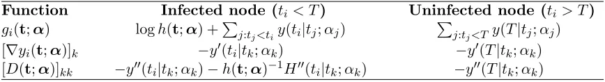
Function Infected node (ti< T) Uninfected node (ti > T)
gi(t;α) logh(t;α) +Pj:tj<tiy(ti|tj;αj) Pj:tj<T y(T|tj;αj)
[∇yi(t;α)]k −y0(ti|tk;αk) −y0(T|tk;αk)
[D(t;α)]kk −y00(ti|tk;αk)−h(t;α)−1H00(ti|tk;αk) −y00(T|tk;αk)
Table 2: Functions. gi(t;α) is nodei’s log-likelihood in a cascadet,yi(t;α) is the logarithm
of nodei’s survivals in a cascadet,D(t;α) is a diagonal matrix defined in Eq. 5,
H(ti|tk;αk) is the hazard function, andh(t;α) denotes the sum of nodei’s hazard
functions in a cascadet.
P(s). Then, the network inference problem consists of finding the directed edges and the associated parameters using only the temporal information from the set of cascadesCn.
This problem has been cast as a maximum likelihood estimation problem (Gomez-Rodriguez et al., 2011)
minimizeA −n1
P
c∈Cnlogf(tc;A)
subject to αji≥0, i, j= 1, . . . , N, i6=j,
(2)
where the inferred edges in the network correspond to those pairs of nodes with non-zero parameters,i.e.αjiˆ >0.
In fact, the problem in Eq. 2 decouples into a set of independent smaller subproblems, one per node, where we infer the parents of each node and the parameters associated with these incoming edges. Without loss of generality, for a particular node i, we solve the problem
minimizeαi ` n(αi)
subject to αji ≥0, j= 1, . . . , N, i6=j, (3)
where the parameters αi := {αji|j = 1, . . . , N, i 6= j} are the relevant variables, and `n(αi) =−n1P
c∈Cngi(tc;αi) corresponds to the terms in Eq. 2 involvingαi. The function g(·;αi) is simple for several well-known parametric transmission likelihoods, including those described in Table 1. For example, for an exponential transmission likelihood,
gi(t;αi) = log
X
j:tj<ti αji
− X
j:tj<ti
αji(ti−tj)
for an infected node and gi(t;αi) = −P
j:tj<T αji(T −tj) for an uninfected node. Refer
to Table 2 for a general definition of g(·;αi). Moreover, in this subproblem, we only need to consider a super-neighborhood Vi =Ri∪ Ui ofi, with cardinality pi =|Vi| ≤ N, where
Ri is the set of upstream nodes from which i is reachable, Ui is the set of nodes which are reachable from at least one node j ∈ Ri. Here, we consider a node i to be reachable
from a node j if and only if there is a directed path from j toi. We can skip all nodes in
V\Vi from our analysis because they will never be infected in a cascade before i, and thus, the maximum likelihood estimation of the associated transmission rates will always be zero (and correct).
recover the true network structure with this approach given a finite amount of cascades and, if so, how many cascades are needed. We will show that by adding an `1-regularizer to the objective function and solving instead the following optimization problem
minimizeαi `
n(αi) +λn||αi||
1
subject to αji ≥0, j= 1, . . . , N, i6=j,
(4)
we can provide finite sample guarantees for recovering the network structure (and parame-ters). Our analysis also shows that by selecting an appropriate value for the regularization parameter λn, the solution of Eq. 4 successfully recovers the network structure with prob-ability approaching 1 exponentially fast inn.
In the remainder of the paper, we will focus on estimating the parent nodes of a particular nodei. For simplicity, we will useα=αi,αj =αji,N−=N−(i),R=Ri,U =Ui,d=di, pi =p and α∗min =α∗min,i.
4. Consistency
Can we recover the hidden network structures from the observed cascades? The answer is yes. We will show this by proving that the estimator provided by Eq. 3 is consistent, meaning that as the number of cascades goes to infinity, we can always recover the true network structure.
More specifically, Gomez-Rodriguez et al. (2011) showed that the network inference problem defined in Eq. 3 is convex in α if the survival functions are log-concave and the hazard functions are concave in α. Under these conditions, the Hessian matrix, Qn =
∇2`n(α), can be expressed as the sum of a nonnegative diagonal matrixDn and the outer
product of a matrix Xn(α) with itself,i.e.,
Qn=Dn(α) +n1Xn(α)[Xn(α)]>. (5) Here the diagonal matrix Dn(α) = 1nP
cD(tc;α) is a sum over a set of diagonal matrices D(tc;α), one for each cascadec (see Table 2 for the definition of its entries); and Xn(α) is the Hazard matrix
Xn(α) =
X(t1;α)|X(t2;α)|. . . |X(tn;α)
, (6)
with each column X(tc;α) := h(tc;α)−1∇αh(tc;α). Intuitively, the Hessian matrix cap-tures the co-occurrence information of nodes in cascades. Both D(tc;α) and Xn(α) are simple for several well-known transmission likelihoods, including those described in Ta-ble 1. For example, for an exponential transmission likelihood, [D(tc;α)]kk = 0 and
[Xn(α)]j =
P
k:tk<tiαki
−1
iftj < ti and 0 otherwise. Then, we can prove the following consistency result:
Theorem 1 If the source probabilityP(s) is strictly positive for all s∈ R, then, the maxi-mum likelihood estimatorαˆ given by the solution of Eq. 3 is consistent.
Proof We check the three criteria for consistency: continuity, compactness and identi-fication of the objective function (Newey and McFadden, 1994). Continuity is obvious. For compactness, since L → −∞ for both αij → 0 and αij → ∞ for all i, j so we lose
Appendices 12.1 and 12.2), which establish that Xn(α) has full row rank as n→ ∞, and henceQn is positive definite.
5. Recovery Conditions
In this section, we will find a set of sufficient conditions on the diffusion model and the cascade sampling process under which we can recover the network structure from finite samples. These results allow us to address two questions:
• Are there some network structures which are more difficult than others to recover?
• What kind of cascades are needed for the network structure recovery?
The answers to these questions are intertwined. The difficulty of finite-sample recovery depends crucially on an irrepresentability condition which is a function of both network structure, parameters of the diffusion model and the cascade sampling process. Intuitively, the sources of the cascades in a diffusion network have to be chosen in such a way that nodes without parent-child relation should co-occur less often compared to nodes with such relation. Many commonly used diffusion models and network structures can be naturally made to satisfy this condition.
More specifically, we first place two conditions on the Hessian of the population log-likelihood, Ec[`n(α)] =Ec[logg(tc;α)], where the expectation here is taken over the
dis-tributionP(s) of the source nodes, and the densityf(tc|s) of the cascadestcgiven a source node s. In this case, we will further denote the Hessian of Ec[logg(tc;α)] evaluated at the
true model parameterα∗ asQ∗. Then, we place two conditions on the Lipschitz continuity ofX(tc;α), and the boundedness ofX(tc;α∗) and∇g(tc;α∗) at the true model parameter
α∗. For simplicity, we will denote the subset of indexes associated to nodei’s true parents asS, and its complement asSc. Then, we useQ∗SS to denote the sub-matrix of Q∗ indexed by S and α∗S the set of parameters indexed byS. Note that α∗Sc = 0.
Condition 1 (Dependency condition): There exists constantsCmin >0 andCmax>
0 such that Λmin(Q∗SS)≥Cmin and Λmax(Q∗SS)≤Cmax where Λmin(·) and Λmax(·) return
the leading and the bottom eigenvalue of its argument respectively. This assumption en-sures that two connected nodes co-occur reasonably frequently in the cascades but are not deterministically related.
Condition 2 (Irrepresentability condition): There exists a constant ε ∈ (0,1] such that |||Q∗ScS(Q∗SS)−1|||∞ ≤1−ε, where |||A|||∞ = maxjPk|Ajk|. This assumption
captures the intuition that, nodeiand any of its neighbors should get infected together in a cascade more often than node iand any of its non-neighbors. A similar irrepresentability condition has been proposed on model selection consistency of Lasso (Zhao and Yu, 2006). Condition 3 (Lipschitz Continuity): For any feasible cascadetc, the Hazard vector
X(tc;α) is Lipschitz continuous in the domain {α:αS ≥α∗min/2},
0
1
2
3 01
12
23
(a) Chain
2
3 1
0
30 10
20
4
5
6
7
41
52
62
73
(b) Tree
1 2 3
p 0
03 02
01
0p
(c) Star
Figure 2: Example networks.
wherek1 is some positive constant. As a consequence, the spectral norm of the difference,
n−1/2(Xn(β)−Xn(α)), is also bounded (refer to appendix 12.3), i.e.,
|||n−1/2 Xn(β)−Xn(α)
|||2≤k1kβ−αk2. (7) Furthermore, for any feasible cascadetc,D(α)jj is Lipschitz continuous for allj∈ V,
|D(tc;β)jj−D(tc;α)jj| ≤k2kβ−αk2, wherek2 is some positive constant.
Condition 4 (Boundedness): For any feasible cascadetc, the absolute value of each entry in the gradient of its log-likelihood and in the Hazard vector, as evaluated at the true model parameter α∗, is bounded,
k∇g(tc;α∗)k∞≤k3, kX(tc;α∗)k∞≤k4,
wherek3andk4 are positive constants. Then the absolute value of each entry in the Hessian matrixQ∗, is also bounded|||Q∗|||
∞≤k5.
Remarks for condition 1 As stated in Theorem 1, as long as the source probability P(s) is strictly positive for alls∈ R, the maximum likelihood formulation is strictly convex and thus there existsCmin >0 such that Λmin(Q∗)≥Cmin. Moreover, condition 4 implies
that there exists Cmax >0 such that Λmax(Q∗)≤Cmax.
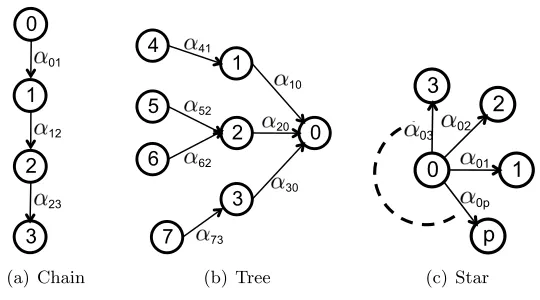
Remarks for condition 2 The irrepresentability condition depends, in a non-trivial way, on the network structure, diffusion parameters, observation window and source node distribution. Here, we give some intuition by studying three small canonical examples.
First, consider the chain graph in Fig. 2(a) and assume that we would like to find the incoming edges to node 3 whenT → ∞. Then, it is easy to show that the irrepresentability condition is satisfied if (P0+P1)/(P0+P1+P2)<1−εandP0/(P0+P1+P2)<1−ε, where
Pi denotes the probability of a node ito be the source of a cascade. Thus, for example, if
the source of each cascade is chosen uniformly at random, the inequality is satisfied. Here, the irrepresentability condition depends on the source node distribution.
Second, consider the directed tree in Fig. 2(b) and assume that we would like to find the incoming edges to node 0 whenT → ∞. Then, it can be shown that the irrepresentability condition is satisfied as long as (1) P1 > 0, (2) (P2 >0) or (P5 >0 and P6 >0), and (3)
Finally, consider the star graph in Fig. 2(c), with exponential edge transmission func-tions, and assume that we would like to find the incoming edges to a leave node i when
T < ∞. Then, as long as the root node has a nonzero probability P0 > 0 of being the source of a cascade, it can be shown that the irrepresentability condition reduces to the inequalities
1−α0iα0j+α0je−(α0i+α0j)T + α0iα0j+α0j <1−ε(1 +e−α0iT), j = 1, . . . , p : j 6=i, which always holds for some ε > 0. If T → ∞, then the condition holds whenever
ε < α0i/(α0i + maxj:j6=iα0j). Here, the larger the ratio maxj:j6=iα0j/α0i is, the smaller
the maximum value ofεfor which the irrepresentability condition holds. To summarize, as long as P0 >0, there is always some ε >0 for which the condition holds, and suchεvalue depends on the time window and the parameters α0j.
Remarks for conditions 3 and 4 Well-known pairwise transmission likelihoods such as exponential, Rayleigh or Power-law, used in previous work Gomez-Rodriguez et al. (2011), satisfy conditions 3 and 4.
6. Sample Complexity
How many cascades do we need to recover the network structure? We will answer this question by providing a sample complexity analysis of the optimization in Eq. 4. Given the conditions spelled out in Section 5, we can show that the number of cascades needs to grow polynomially in the number of true parents of a node, and depends only logarithmically on the size of the network. This is a positive result, since the network size can be very large (millions or billions), but the number of parents of a node is usually small compared the network size. More specifically, for each individual node, we have the following result:
Theorem 2 Consider an instance of the continuous-time diffusion model with parameters
αji∗ and associated edges E∗ such that the model satisfies condition 1-4, and let Cn be a set of n cascades drawn from the model. Suppose that the regularization parameter λn is
selected to satisfy
λn≥8k3 2−ε
ε
r
logp
n . (8)
Then, there exist positive constantsL and K, independent of (n, p, d), such that if
n > Ld3logp, (9)
then the following properties hold with probability at least 1−2 exp(−Kλ2
nn):
1. For each nodei∈ V, the`1-regularized network inference problem defined in Eq. 4 has a unique solution, and so uniquely specifies a set of incoming edges of node i.
2. For each node i∈ V, the estimated set of incoming edges does not include any false edges and include all true edges.
Furthermore, suppose that the finite sample Hessian matrixQn satisfies conditions 1 and 2.
Then there exist positive constantsL and K, independent of (n, p, d), such that the sample complexity can be improved to n > Ld2logp with other statements remain the same.
except that the dependency ondwill change fromdtodmax (the largest number of parents
of a node), and the dependency on p will change from logp to 2 logN (N the number of nodes in the network).
6.1 Outline of Analysis
The proof of Theorem 2 uses a technique called primal-dual witness method, previously used in the proof of sparsistency of Lasso (Wainwright, 2009) and high-dimensional Ising model selection (Ravikumar et al., 2010). To the best of our knowledge, the present work is the first that uses this technique in the context of diffusion network inference. First, we show that the optimal solutions to Eq. 4 have shared sparsity pattern, and under a further condition, the solution is unique (proven in Appendix 12.4):
Lemma 3 Suppose that there exists an optimal primal-dual solution(α,ˆ µˆ)to Eq. 4 with an associated subgradient vectorˆz such that ||ˆzSc||∞ <1. Then, any optimal primal solution
˜
α must haveαS˜ c = 0. Moreover, if the Hessian sub-matrix QnSS is strictly positive definite,
thenαˆ is the unique optimal solution.
Next, we will construct a primal-dual vector (α,ˆ µˆ) along with an associated subgradient vector ˆz. Furthermore, we will show that, under the assumptions on (n, p, d) stated in Theorem 2, our constructed solution satisfies the KKT optimality conditions to Eq. 4, and the primal vector has the same sparsity pattern as the true parameterα∗,i.e.,
ˆ
αj >0, ∀j:αj∗>0, (10)
ˆ
αj = 0, ∀j:αj∗= 0. (11)
Then, based on Lemma 3, we can deduce that the optimal solution to Eq. 4 correctly recovers the sparsisty pattern ofα∗, and thus the incoming edges to nodei.
More specifically, we start by realizing that a primal-dual optimal solution (α,˜ µ˜) to Eq. 4 must satisfy the generalized Karush-Kuhn-Tucker (KKT) conditions Boyd and Van-denberghe (2004):
0∈ ∇`n(α˜) +λn˜z−µ,˜ (12)
˜
µjα˜j = 0, (13)
˜
µj ≥0, (14)
˜
zj = 1, ∀αj˜ >0, (15)
|zj˜| ≤1, ∀αj˜ = 0, (16) where`n(α˜) =−1
n
P
c∈Cnlogg(tc;α˜) and˜z denotes the subgradient of the `1-norm. Suppose the true set of parent of nodeiisS. We construct the primal-dual vector (α,ˆ µˆ) and the associated subgradient vectorˆz in the following way
1. We set αˆS as the solution to the partial regularized maximum likelihood problem
ˆ
αS = argmin (αS,0),αS≥0
2. We set αˆSc = 0, so that condition (11) holds, and µˆSc = µ∗Sc ≥ 0, where µ∗ is the
optimal dual solution to the following problem:
minimizeα Ec[`n(α)]
subject to αj ≥0, j= 1, . . . , N, i6=j. (18)
Thus, our construction satisfies condition (14).
3. We obtainˆzSc from (12) by substituting in the constructedαˆ,µˆ andˆzS.
Then, we only need to prove that, under the stated scalings of (n, p, d), with high-probability, the remaining KKT conditions (10), (13), (15) and (16) hold.
For simplicity of exposition, we first assume that the dependency and irrepresentability conditions hold for the finite sample Hessian matrix Qn. Later we will lift this restriction
and only place these conditions on the population Hessian matrixQ∗. The following lemma (proven in Appendix 12.5) show that our constructed solution satisfies condition (10):
Lemma 4 Under condition 3, if the regularization parameter is selected to satisfy
√
dλn≤ C
2 min 6(k2+ 2k1
√
Cmax)
,
and k∇s`n(α∗)k∞≤ λn4 , then,
kαSˆ −α∗Sk2 ≤
3√dλn Cmin
≤ α
∗ min
2 ,
as long as α∗min ≥6√dλn/Cmin.
Based on this lemma, we can then further show that the KKT conditions (13) and (15) also hold for the constructed solution. This can be trivially deduced from condition (10) and (11), and our construction steps (a) and (b). Note that it also implies that µˆS =µ∗S = 0,
and henceµˆ=µ∗.
Proving condition (16) is more challenging. We first provide more details on how to constructˆzSc mentioned in step (c). We start by using a Taylor expansion of Eq. 12,
Qn(αˆ−α∗) =−∇`n(α∗)−λnzˆ+µˆ−Rn, (19) whereRn is a remainder term with its j-th entry
Rnj =
∇2`n(α¯
j)− ∇2`n(α∗)
T
j(αˆ−α
∗),
andαj¯ =θjαˆ+ (1−θj)α∗ withθj ∈[0,1] according to the mean value theorem. Rewriting Eq. 19 using block matrices
Qn
SS QnSSc
Qn
ScS QnScSc
ˆ
αS−α∗S
ˆ
αSc−α∗Sc
=−
∇S`n(α∗)
∇Sc`n(α∗)
−λn
ˆ
zS
ˆ
zSc
+
ˆ
µS
ˆ
µSc
−
RnS RnSc
(20)
and, after some algebraic manipulation, we have
λˆzSc =−∇Sc`n(α∗) +µSˆ c−RnSc− QnScS(QnSS)−1 − ∇s`n(α∗)−λzSˆ +µSˆ −RnS
. (21)
Next, we upper boundkˆzSck∞using the triangle inequality
kˆzSck∞ ≤λ−n1kµ∗Sc− ∇Sc`n(α∗)k∞+λ−n1kRnSck∞+kQnScS(QnSS)−1k∞×1 +λ−n1kRnSk∞ +λ−n1kµ∗S− ∇S`n(α∗)k∞
and we want to prove that this upper bound is smaller than 1. This can be done with the help of the following two lemmas (proven in Appendices 12.6 and 12.7):
Lemma 5 Given ε∈(0,1]from the irrepresentability condition, we have,
P
2−ε
λn k∇`
n(α∗
)−µ∗k∞≥4−1ε
≤2pexp − nλ
2
nε2
32k2
3(2−ε) 2
!
, (22)
which converges to zero at rate exp(−cλ2nn) as long as λn≥8k32−εε
q
logp
n .
Lemma 6 Givenε∈(0,1]from the irrepresentability condition, if conditions 3 and 4 holds,
λn is selected to satisfy
λnd≤Cmin2 ε
36K(2−ε),
where K =k1+k4k1+k12+k1
√
Cmax, and k∇s`n(α∗)k∞ ≤ λn4 , then, kR
nk ∞
λn ≤
ε
4(2−ε), as long as α∗min≥6√dλn/Cmin.
Now, applying both lemmas and the irrepresentability condition on the finite sample Hessian matrixQn, we have
kˆzSck∞ ≤ (1−ε) +λ−n1(2−ε)kRnk∞ +λ−n1(2−ε)kµ∗− ∇`n(α∗)k∞
≤ (1−ε) + 0.25ε+ 0.25ε= 1−0.5ε,
and thus condition (16) holds.
A possible choice of the regularization parameter λn and cascade set size n such that the conditions of the Lemmas 4-6 are satisfied is λn = 8k3(2−ε)ε−1
p
n−1logp and n > 2882k32(2−ε)4Cmin−4 ε−4d2logp+ 48k3(2−ε)Cmin−1 (α∗min)−1ε−1
2
dlogp.
Last, we lift the dependency and irrepresentability conditions imposed on the finite sample Hessian matrixQn. We show that if we only impose these conditions in the
corres-ponding population matrixQ∗, then they will also hold forQnwith high probability (proven
in Appendices 12.8 and 12.9).
Lemma 7 If condition 1 holds for Q∗, then, for anyδ >0,
P(Λmin(QnSS)≤Cmin−δ)≤2dB1exp
−A1
δ2n d2
,
P(Λmax(QnSS)≥Cmax+δ)≤2dB2exp
−A2
δ2n d2
,
where A1,A2, B1 and B2 are constants independent of (n, p, d). Lemma 8 If |||Q∗
ScS(Q∗SS)
−1|||
∞≤1−ε, then,
P kQn
ScS(QnSS)−1k∞≥1−ε/2≤pexp
−Kn d3
,
where K is a constant independent of (n, p, d).
Algorithm 1 `1-regularized network inference Require: Cn, λn, K, L
for all i∈ V do
k= 0
whilek < K do
αki+1 = αki −L∇αi` n(αk
i)−λnL
+
k=k+ 1 end while
ˆ
αi =αKi −1 end for
return {αˆi}i∈V
7. Efficient soft-thresholding algorithm
Can we design efficient algorithms to solve Eq. (4) for network recovery? Here, we will design a proximal gradient algorithm which is well suited for solving non-smooth, con-strained, large-scale or high-dimensional convex optimization problems Parikh and Boyd (2013). Moreover, they are easy to understand, derive, and implement. We first rewrite Eq. 4 as an unconstrained optimization problem:
minimizeα `n(α) +g(α),
where the non-smooth convex function g(α) = λn||α||1 if α ≥0 and +∞ otherwise. By rewriting both problems as a sum of a smooth convex function `n(α) and a non-smooth
convex functiong(α), the general recipe from Parikh and Boyd (2013) for designing proximal gradient algorithm can be applied directly.
Algorithm 1 summarizes the resulting algorithm. In each iteration of the algorithm, we need to compute ∇`n (Table 2) and the proximal operator proxLkg(v), where Lk is a
step size that we can set to a constant value Lor find using a simple line search Beck and Teboulle (2009). Using Moreau’s decomposition, we have
proxLkg(v) =v−Lk proxg∗/Lk(v/Lk), (23)
where
g∗(y) = sup
x
(y−λn1)Tx−1(x≥0)
=
∞ if∃i:yi > λn
0 otherwise is the conjugate function ofg. Then,
proxg∗/Lk(v/Lk) = argmin y
{g∗(y) +L
k
2 ky−v/L
kk2
2}= (v−λnLk)+
In summary, the proximal operator for our particular functiong(·) is a soft-thresholding operator, (v−λnLk)+, which leads to a sparse optimal solution αˆ, as desired.
8. Experiments
In this section, we first illustrate some consequences of Th. 2 by applying our algorithm to several types of networks, parameters (n, p, d), and regularization parameterλn. Then,
we compare our algorithm to two different state-of-the-art algorithms: NetRate
0 0.5 1 1.5 2 0
0.2 0.4 0.6 0.8 1
β
Success Probability
p=6 p=26 p=40
(a) Super-neighborhoodpi
0.4 0.8 1.2 1.6 2 0
0.2 0.4 0.6 0.8 1
β
Source Probability d=1d=2 d=3
(b) In-degreesdi
0 10 20 30 40 50 60
0.2 0.4 0.6 0.8 1
K
Success Probability
Forest−Fire (Exp) Forest−Fire (Pow) Hierarchical (Exp) Hierarchical (pow)
(c)λn
Figure 3: Success probability vs. # of cascades.
Experimental Setup We focus on synthetic networks that mimic the structure of real-world diffusion networks – in particular, social networks. We consider two models of directed real-world social networks: the Forest Fire model (Barab´asi and Albert, 1999) and the Kronecker Graph model (Leskovec et al., 2010), and use simple pairwise transmission models such as exponential, power-law or Rayleigh. We use networks with 128 nodes and, for each edge, we draw its associated transmission rate from a uniform distributionU(0.5,1.5). In general, we proceed as follows: we generate a network G∗ and transmission rates A∗, simulate a set of cascades and, for each cascade, record the node infection times. Then, given the infection times, we infer a network ˆG. Finally, when we illustrate the consequences of Th. 2, we evaluate the accuracy of the inferred neighborhood of a node ˆN−(i) using probability of success P( ˆE = E∗), estimated by running our method of 100 independent cascade sets. When we compare our algorithm toNetRateand First-Edge, we use theF1 score, which is defined as 2P R/(P+R), where precision (P) is the fraction of edges in the inferred network ˆG present in the true networkG∗, and recall (R) is the fraction of edges of the true networkG∗ present in the inferred network ˆG.
Parameters (n, p, d) According to Th. 2, the number of cascades that are necessary to successfully infer the incoming edges of a node will increase polynomially to the node’s neighborhood sizedi and logarithmically to the super-neighborhood size pi. Here, we first infer the incoming links of nodes on the same type of canonical networks as depicted in Fig. 2. We choose nodes the same in-degree but different super-neighboorhod set sizes pi
and experiment with different scalings β of the number of cascades n = 10βdlogp. We set the regularization parameter λn as a constant factor of
p
log(p)/n as suggested by Theorem 2 and, for each node, we used cascades which contained at least one node in the super-neighborhood of the node under study. We used an exponential transmission model and time windowT = 10. As predicted by Theorem 2, very differentpvalues lead to curves that line up with each other quite well.
Next, we infer the incoming links of nodes of a larger hierarchical Kronecker network. Again, we choose nodes with the same in-degree (di = 3) but different super-neighboorhod
set sizes pi under different scalings β of the number of cascades n= 10βdlogp. We used an exponential transmission model andT = 5. Fig. 3(a) summarizes the results, where, for each node, we used cascades which contained at least one node in the super-neighborhood of the node under study. Similarly as in the case of the canonical networks, very different
0.1 0.2 0.3 0.4 0.5 0.4
0.5 0.6 0.7 0.8 0.9 1
β
Success Probability
P=16 P=32 P=64 P=128 P=256
(a) Chain (di= 1)
0 0.2 0.4 0.6 0.8 1 0
0.2 0.4 0.6 0.8 1
β
Success Probability
p=31 p=63 p=127
(b) Stars (di= 1)
0 0.02 0.04 0.06 0.08 0.1
0 0.2 0.4 0.6 0.8 1
β
Sucess Probability p=39p=120
p=363
(c) Tree (di= 3)
Figure 4: Success probability vs. # of cascades. Different super-neighborhood sizespi.
Finally, we infer the incoming links of nodes of a hierarchical Kronecker network with equal super neighborhood size (pi = 70) but different in-degree (di) under different scalings β of the number of cascades n = 10βdlogp and choose the regularization parameter λn
as a constant factor of plog(p)/n as suggested by Theorem 2. We used an exponential transmission model and time window T = 5. Figure 3(b) summarizes the results, where we observe that, as predicted by Theorem 2, different dvalues lead to noticeably different curves.
Regularization parameter λn Our main result indicates that the regularization
parameter λn should be a constant factor of
p
log(p)/n. Fig. 3(c) shows the success probability of our algorithm against different scalings K of the regularization parameter
λn= K
p
log(p)/n for different types of networks using 150 cascades and T = 5. We find that for sufficiently large λn, the success probability flattens, as expected from Th. 2. It
flattens at values smaller than one because we used a fixed number of cascades n, which may not satisfy the conditions of Th. 2.
Comparison with NetRate and First-Edge Fig. 5 compares the accuracy of our algorithm, NetRate and First-Edge against number of cascades for three hierarchical
Kronecker network and three Forest Fire networks, with power-law (Pow), exponential
(Exp) and rayleigh (Ray) transmission models, and an observation window T = 10. Our
method outperforms both competitive methods, finding especially striking the competitive advantage with respect to First-Edge, however, this may be explained by comparing the sample complexity results for both methods: First-Edge needs O(N dlogN) cascades to achieve a probability of success approaching 1 in a rate polynomial in the number of cascades while our method needs O(d3logN) to achieve a probability of success approaching 1 in a rate exponential in the number of cascades.
9. Discussion
500 1000 1500 2000 2500 0.5 0.6 0.7 0.8 0.9 1 # cascades F1 NetRate Our method First Edge
(a) Kronecker Hier.,Pow
500 1000 1500 2000 2500 0.5 0.6 0.7 0.8 0.9 1 # cascades F1 NetRate Our method First Edge
(b) Kronecker Hier.,Exp
500 1000 1500 2000 2500 0.5 0.6 0.7 0.8 0.9 1 # cascades F1 NetRate Our method First Edge
(c) Kronecker Hier., Ray
500 1000 1500 2000 2500 0.5 0.6 0.7 0.8 0.9 1 # cascades F1 NetRate Our method First Edge
(d) Forest Fire,Pow
500 1000 1500 2000 2500 0.5 0.6 0.7 0.8 0.9 1 # cascades F1 NetRate Our method First Edge
(e) Forest Fire,Exp
500 1000 1500 2000 2500
0.5 0.6 0.7 0.8 0.9 # cascades F1 NetRate Our method First Edge
(f) Forest Fire, Ray
Figure 5: F1-score vs. # of cascades.
et al., 2012a), transmission function conditioned on additional features (Du et al., 2013), diffusion models which allows for multiple events (Zhou et al., 2013). All three models will result in convex loss function; and for the former two models, we can employ grouped lasso regularization (Yuan and Lin, 2006), while for the latter model, we can employ a nuclear norm regularization (Recht et al., 2010). These models are more complicated than the independent cascade model we studied in the paper, but analysis for these models can be carried out using a general M-estimation analysis framework (Negahban et al., 2009), since these regularizers are decomposable and one needs to check the restricted strong convex-ity of the loss function. In terms of the estimation algorithms, we can employ proximal algorithms (Parikh and Boyd, 2013) or the conditional gradient algorithm (Jaggi, 2013) to deal with different type of diffusion models and regularizers. When the data is large, one can consider distributed (Boyd et al., 2011) and online estimation (Nemirovski et al., 2009) procedures.
Our results also bring out interesting further open problems on diffusion network es-timations. For instance, the success of the network inference algorithm in Equation (2) relies on the fulfillment of the above mentioned irrepresentability condition on the Hessian,
Q∗, of the population log-likelihood
the source locations to sample from may be determined actively in a sequential manner, potentially based on the information gathered from previous source locations. Thus an interesting open question is:
Suppose there exists an unknown P(s) where the irrepresentability conditions hold for the diffusion model. Under what conditions, can we design an “active” algorithm which samples the source location intelligently and achieves the sample complexity in Theorem 2, or even better sample complexity,e.g.,o(d3i logN)?
10. Conclusions
Our work contributes towards establishing a theoretical foundation of the network inference problem. Specifically, we proposed a `1-regularized maximum likelihood inference method for a well-known continuous-time diffusion model and an efficient proximal gradient imple-mentation, and then show that, for general networks satisfying a natural irrepresentability condition, our method achieves an exponentially decreasing error with respect to the number of cascades as long as O(d3logN) cascades are recorded.
Our work also opens many interesting venues for future work. For example, given a fixed number of cascades, it would be useful to provide confidence intervals on the inferred edges. Further, a detailed theoretical analysis of the irrepresentability condition on large synthetic networks that mimic the structure of real-world diffusion networks, such as Kronecker or Forest-Fire networks, is still missing. Given a network with arbitrary pairwise likelihoods, it is an open question whether there always exists at least one source distribution and time window value such that the irrepresentability condition is satisfied, and, and if so, whether there is an efficient way of finding this distribution. Finally, our work assumes all activations occur due to network diffusion and are recorded. It would be interesting to allow for missing observations, as well as activations due to exogenous factors.
11. Acknowledgement
This research was supported in part by NSF/NIH BIGDATA 1R01GM108341-01, NSF IIS1116886, NSF CAREER IIS-1350983 and a Raytheon faculty fellowship to L. Song.
12. Appendix
12.1 Proof of Lemma 9
Lemma 9 Given log-concave survival functions and concave hazard functions in the param-eter(s) of the pairwise transmission likelihoods, then, a sufficient condition for the Hessian matrix Qn to be positive definite is that the hazard matrix Xn(α) is non-singular.
12.2 Proof of Lemma 10
Lemma 10 If the source probability P(s) is strictly positive for all s ∈ R, then, for an arbitrarily large number of cascades n → ∞, there exists an ordering of the nodes and cascades within the cascade set such that the hazard matrix Xn(α) is non-singular.
Proof In this proof, we find a labeling of the nodes (row indices in Xn(α)) and ordering
of the cascades (column indices in Xn(α)), such that, for an arbitrary large number of cascades, we can express the matrixXn(α) as [T B], whereT ∈Rp×p is an upper triangular
with nonzero diagonal elements and B ∈ Rp×n−p. And, therefore, Xn(α) has full rank (rankp). We proceed first by sorting nodes inR and then continue by sorting nodes in U:
• Nodes in R: For each nodeu∈ R, consider the set of cascades Cu in whichu was a source and igot infected. Then, rank each node u according to the earliest position in which node i got infected across all cascades in Cu in decreasing order, breaking
ties at random. For example, if a nodeu was, at least once, the source of a cascade in which nodeigot infected just after the source, but in contrast, node vwas never the source of a cascade in which node i got infected the second, then nodeu will have a lower index than nodev. Then, assign rowkin the matrixXn(α) to node in position
k and assign the first d columns to the corresponding cascades in which node i got infected earlier. In such ordering,Xn(α)mk = 0 for allm < k and Xn(α)kk6= 0.
• Nodes in U: Similarly as in the first step, and assign them the rows d+ 1 to p. Moreover, we assign the columns d+ 1 to p to the corresponding cascades in which node i got infected earlier. Again, this ordering satisfies that Xn(α)mk = 0 for all m < k and Xn(α)kk 6= 0. Finally, the remaining columns n−p can be assigned to
the remaining cascades at random.
This ordering leads to the desired structure [T B], and thus it is non-singular.
12.3 Proof of Eq 7.
If the Hazard vector X(tc;α) is Lipschitz continuous in the domain{α:αS ≥ α∗min
2 },
kX(tc;β)−X(tc;α)k2 ≤k1kβ−αk2,
wherek1is some positive constant. Then, we can bound the spectral norm of the difference, 1
√
n(X
n(β)−Xn(α)), in the domain{α:αS ≥ α∗min
2 } as follows:
|k√1
n X
n(β)−Xn(α)
k|2= max kuk2=1
1
√
nku X
n(β)−Xn(α)
k2
= max kuk2=1
1
√
n
v u u t
n
X
c=1
hu,X(tc;β)−X(tc;α)i2≤ √1
n
q
k2
12.4 Proof of Lemma 3
By Lagrangian duality, the regularized network inference problem defined in Eq. 4 is equiv-alent to the following constrained optimization problem:
minimizeαi ` n(αi)
subject to αji ≥0, j= 1, . . . , N, i6=j,
||αi||1 ≤C(λn)
(24)
whereC(λn)<∞is a positive constant. In this alternative formulation,λnis the Lagrange
multiplier for the second constraint. Since λn is strictly positive, the constraint is active at any optimal solution, and thus||αi||1 is constant across all optimal solutions.
Using that `n(αi) is a differentiable convex function by assumption and {α : αji ≥
0,||αi||1 ≤C(λn)}is a convex set, we have that∇`n(αi) is constant across optimal primal solutions Mangasarian (1988). Moreover, any optimal primal-dual solution in the original problem must satisfy the KKT conditions in the alternative formulation defined by Eq. 24, in particular,
∇`n(αi) =−λnz+µ,
whereµ≥0 are the Lagrange multipliers associated to the non negativity constraints and z denotes the subgradient of the `1-norm.
Consider the solution αˆ such that ||ˆzSc||∞ <1 and thus∇αSc`n(αˆi) =−λnˆzSc+µˆSc.
Now, assume there is an optimal primal solution α˜ such that ˜αji > 0 for some j ∈ Sc, then, using that the gradient must be constant across optimal solutions, it should hold that −λnzˆj + ˆµj = −λn, where ˜µji = 0 by complementary slackness, which implies ˆµj =
−λn(1−zjˆ) < 0. Since ˆµj ≥ 0 by assumption, this leads to a contradiction. Then, any primal solution α˜ must satisfy α˜Sc = 0 for the gradient to be constant across optimal
solutions.
Finally, sinceαSc = 0 for all optimal solutions, we can consider the restricted
optimiza-tion problem defined in Eq. 17. If the Hessian sub-matrix [∇2L(αˆ)]
SS is strictly positive
definite, then this restricted optimization problem is strictly convex and the optimal solution must be unique.
12.5 Proof of Lemma 4
To prove this lemma, we will first construct a function
G(uS) :=`n(α∗S+uS)−`n(α∗S) +λn(kα ∗
S+uSk1− kα∗Sk1).
whose domain is restricted to the convex set U = {uS :α∗S+uS ≥ 0}. By construction, G(uS) has the following properties
1. It is convex with respect touS.
2. Its minimum is obtained atuSˆ :=αSˆ −α∗S. That isG(uSˆ )≤G(uS),∀uS 6=uSˆ .
3. G(uSˆ )≤G(0) = 0.
Based on the properties 1 and 3 above, we deduce that any point in the segment, L :=
{uS˜ :uS˜ =tuSˆ + (1−t)0, t∈[0,1]}, connecting uSˆ and 0 hasG(uS˜ )≤0. That is
Next, we will find a sphere centered at 0 with strictly positive radius B, S(B) :=
{uS :kuSk2=B}, such that function G(uS) > 0 (strictly positive) on S(B). We note that this sphereS(B) can not intersect with the segmentL since the two sets have strictly different function values. Furthermore, the only possible configuration is that the segment is contained inside the sphere entirely, leading us to conclude that the end pointuSˆ :=αSˆ −α∗S
is also within the sphere. That iskαˆS−α∗Sk2≤B.
In the following, we will provide details on finding such a suitable B which will be a function of the regularization parameterλn and the neighborhood sized. More specifically,
we will start by applying a Taylor series expansion and the mean value theorem,
G(uS) =∇S`n(α∗S)
>
uS+u>S∇2SS`n(α
∗
S+buS)uS+λn(kαS∗ +uSk1− kα∗Sk1), (25) where b ∈ [0,1]. We will show that G(uS) > 0 by bounding below each term of above
equation separately.
We bound the absolute value of the first term using the assumption on the gradient,
∇S`(·),
|∇S`n(α∗S)>uS| ≤ k∇S`k∞kuSk1 ≤ k∇S`k∞
√
dkuSk2≤4−1λnB
√
d. (26)
We bound the absolute value of the last term using the reverse triangle inequality.
λn|kα∗S+uSk1− kα∗Sk1| ≤λnkuSk1 ≤λn
√
dkuSk2. (27)
Bounding the remaining middle term is more challenging. We start by rewriting the Hessian as a sum of two matrices, using Eq. 5,
q= min
uS u
>
SDnSS(α∗S+buS)uS+n−1u>SXSn(α∗S+buS)XSn(α∗S+buS)>uS
= min
uS u
>
SDnSS(α
∗
S+buS)uS+ku>SXnS(α
∗
S+buS)k22.
Now, we introduce two additional quantities,
∆DnSS =DnSS(αS∗ +buS)−DnSS(α
∗
S) and ∆XnS =XnS(α
∗
S+buS)−XnS(α
∗
S),
and rewriteq as
q = min
uS
u>SDnSS(α∗S)uS+n−1ku>SXnS(α
∗
S)k22+n −1ku>
S∆XnSk22+u >
S∆DnSSuS
+ 2n−1hu>SXnS(α∗S),u>S∆XnSi
.
Next, we use dependency condition,
q ≥CminB2−max
uS |u
>
S∆DnSSuS
| {z }
T1
| −max
uS 2|n
−1hu>
SXnS(α∗S),u>S∆XnSi
| {z }
T2
|,
and proceed to bound T1 and T2 separately. First, we boundT1 using the Lipschitz condi-tion,
|T1|=|
X
k∈S
u2k[Dnk(α∗S+buS)−Dnk(α
∗
S)]| ≤
X
k∈S
Then, we use the dependency condition, the Lipschitz condition and the Cauchy-Schwartz inequality to boundT2,
T2 ≤ 1
√
nku
>
SXnS(α∗S)k2 1
√
nku
>
S∆XnSk2 ≤
p
CmaxB 1
√
nku
>
S∆XnSk2
≤pCmaxBkuSk2 1
√
n|k∆X n Sk|2≤
p
CmaxB2k1kbuSk2
≤k1
p
CmaxB3,
where we note that applying the Lipschitz condition implies assumingB < αmin2 . Next, we incorporate the bounds of T1 and T2 to lower boundq,
q ≥CminB2−(k2+ 2k1
p
Cmax)B3. (28)
Now, we setB =Kλn
√
d, whereK is a constant that we will set later in the proof, and select the regularization parameter λn to satisfy
λn
√
d≤ Cmin
2K(k2+ 2k1
p
Cmax)
. (29)
Then,
G(uS)≥ −4−1λn
√
dB+ 0.5CminB2−λn
√
dB≥B(0.5CminB−1.25λn
√
d)
≥B(0.5CminKλn
√
d−1.25λn
√
d).
In the last step, we set the constant K = 3Cmin−1, and we have
G(uS)≥0.25λn
√
d >0,
as long as
√
dλn≤ C
2 min 6(k2+ 2k1
√
Cmax)
α∗min≥ 6λn √
d Cmin
.
Finally, convexity of G(uS) yields
kαSˆ −α∗Sk2 ≤3λn
√
d/Cmin ≤
α∗min
2 .
12.6 Proof of Lemma 5
Definezjc= [∇g(tc;α∗)]j and zj = n1 Pczjc. Now, using the KKT conditions and condition
4 (Boundedness), we have that µ∗j =Ec{zjc} and |zjc| ≤ k3, respectively. Thus, Hoeffding’s inequality yields
P
|zj −µ∗j|> λnε
4(2−ε)
≤2 exp − nλ
2
nε2
32k32(2−ε)2
!
,
and then,
P
kz−µ∗k∞>
λnε
4(2−ε)
≤2 exp − nλ
2
nε2
32k2
3(2−ε))
2 + logp
!
12.7 Proof of Lemma 6
We start by factorizing the Hessian matrix, using Eq. 5,
Rnj =∇2`n(αj¯ )− ∇2`n(α∗)>j (αˆ−α∗) =ωjn+δnj,
where,
ωjn=
Dn(α¯j)−Dn(α∗)
>
j (αˆ−α
∗)
δjn= 1
nV n
j (αˆ−α ∗
)
Vjn= [Xn(αj¯ )]jXn(αj¯ )>−[Xn(α∗)]jXn(α∗)>.
Next, we proceed to bound each term separately. Since [αj¯ ]S =θjαSˆ + (1−θj)α∗Swhere θj ∈[0,1], and kαSˆ −α∗Sk∞ ≤ α
∗ min
2 (Lemma 4), it holds that [αj¯ ]S ≥
α∗min
2 . Then, we can use condition 3 (Lipschitz Continuity) to bound ωnj.
|ωnj| ≤k1kαj¯ −α∗k2kαˆ−α∗k2 ≤k1θjkαˆ−α∗k22 ≤k1kαˆ−α∗k22.
However, bounding term δnj is more difficult. Let us start by rewritingδnj as follows.
δjn= (Λ1+Λ2+Λ3) (αˆ−α∗), where,
Λ1 = [Xn(α∗)]j(Xn(αj¯ )>−Xn(α∗)>)
Λ2 ={[Xn(αj¯ )]j−[Xn(α∗)]j}(Xn(αj¯ )>−Xn(α∗)>)
Λ3 = [Xn(αj¯ )]j−[Xn(α∗)]j
Xn(α∗)>.
Next, we bound each term separately. For the first term, we first apply Cauchy inequal-ity,
|Λ1(αˆ−α∗)| ≤ k[Xn(α∗)]jk2× |kXn(α¯j)>−Xn(α∗)>k|2kαˆ−α∗k2, and then use condition 3 (Lipschtiz Continuity) and 4 (Boundedness),
|Λ1(αˆ−α∗)| ≤nk4k1kα¯j−α∗k2kαˆ−α∗k2≤nk4k1kαˆ−α∗k22. For the second term, we also start by applying Cauchy inequality,
|Λ2(αˆ−α∗)| ≤ k[Xn(α¯j)]j−[Xn(α∗)]jk2× |kXn(α¯j)>−Xn(α∗)>k|2kαˆ−α∗k2, and then use condition 3 (Lipschtiz Continuity),
|Λ2(αˆ−α∗)| ≤nk12kαˆ−α∗k22.
Last, for third term, once more we start by applying Cauchy inequality,
|Λ3(αˆ−α∗)| ≤ k[Xn(α¯j)]j−[Xn(α∗)]jk2× |kXn(α∗)>k|2kαˆ−α∗k2,
and then apply condition 1 (Dependency Condition) and condition 3 (Lipschitz Continuity),
|Λ3(αˆ−α∗)| ≤nk1
p
Cmaxkαˆ−α∗k22 Now, we combine the bounds,
kRnk∞≤Kkαˆ −α∗k22, where
K=k1+k4k1+k12+k1
p
Finally, using Lemma 4 and selecting the regularization parameter λn to satisfyλnd≤ Cmin2 36K(2ε−ε) yields:
kRnk∞
λn
≤ 3Kλnd
C2 min
≤ ε
4(2−ε)
12.8 Proof of Lemma 7
We will first bound the difference in terms of nuclear norm between the population Fisher information matrix QSS and the sample mean cascade log-likelihood QnSS. Define zjkc =
[∇2g(tc;α∗) − ∇2`n(α∗)]
jk and zjk = n1Pnc=1zjkc . Then, we can express the difference
between the population Fisher information matrix QSS and the sample mean cascade
log-likelihood Qn
SS as:
|kQnSS(α∗)− Q∗SS(α∗)k|2≤ |kQnSS(α
∗)− Q∗
SS(α
∗)k|
F =
v u u t
d
X
j=1
d
X
k=1 (zik)2.
Since |zjk(c)| ≤2k5 by condition 4, we can apply Hoeffding’s inequality to eachzjk, P(|zjk| ≥β)≤2 exp
−β
2n 8k52
, (30)
and further,
P(|kQnSS(α∗)− Q∗SS(α∗)k|2≥δ)≤2 exp −K
δ2n
d2 + 2 logd
(31)
whereβ2 =δ2/d2. Now, we bound the maximum eigenvalue of Qn
SS as follows:
Λmax(QnSS) = max
kxk2=1
x>QnSSx= max kxk2=1
{x>Q∗SSx+x>(QnSS− Q∗SS)x}
≤y>Q∗SSy+y>(QnSS − Q∗SS)y,
wherey is unit-norm maximal eigenvector of Q∗SS. Therefore, Λmax(QnSS)≤Λmax(Q∗SS) +|kQnSS− Q∗SSk|2, and thus,
P Λmax(QnSS)≥Cmax+δ
≤exp
−Kδ
2n
d2 + 2 logd
.
Reasoning in a similar way, we bound the minimum eigenvalue ofQn SS:
P Λmin(QnSS)≤Cmin−δ
≤exp
−Kδ
2n
d2 + 2 logd
12.9 Proof of Lemma 8
We start by decomposingQn
ScS(α∗)(QSncS(α∗))−1 as follows:
where,
A1=Q∗ScS[(QnScS)−1−(Q∗ScS)−1],
A2= [QnScS− Q∗ScS][(QSncS)−1−(Q∗ScS)−1] A3= [QnScS− QS∗cS](Q∗SS)−1,
A4=Q∗ScS(Q∗SS)−1,
Q∗ =Q∗(α∗) andQn =Qn(α∗). Now, we bound each term separately. The fourth term, A4, is the easiest to bound, using simply the incoherence condition:
|kA4k|∞≤1−ε. To bound the other terms, we need the following lemma:
Lemma 11 For any δ≥0 and constants K and K0, the following bounds hold:
P[|kQnScS− QS∗cSk|∞≥δ]≤2 exp
−Knδ
2
d2 + logd+log(p−d)
(32)
P[|kQnSS− Q∗SSk|∞≥δ]≤2 exp
−Knδ
2
d2 + 2 logd
(33)
P[|k(QnSS)−1−(Q∗SS)−1k|∞≥δ]≤4 exp
−Knδ d3 −K
0logd
(34)
Proof We start by proving the first confidence interval. By definition of infinity norm of a matrix, we have:
P[|kQnScS− Q∗ScSk|∞≥δ] =Pmax
j∈Sc
X
k∈S
|zjk| ≥δ≤(p−d)P X k∈S
|zjk| ≥δ,
wherezjk = [Qn− Q∗]
jk and, for the last inequality, we used the union bound and the fact
that|Sc| ≤p−d. Furthermore,
P X
k∈S
|zjk| ≥δ≤P[∃k∈S||zjk| ≥δ/d]≤dP[|zjk| ≥δ/d].
Thus,
P[|kQnScS− Q∗ScSk|∞≥δ]≤(p−d)dP[|zjk| ≥δ/d].
At this point, we can obtain the first confidence bound by using Eq. 30 with β=δ/din the above equation. The proof of the second confidence bound is very similar and we omit it for brevity. To prove the last confidence bound, we proceed as follows:
|k(QnSS)−1−(QSS∗ )−1k|∞=|k(QnSS)
−1[Qn
SS− Q
∗
SS](Q
∗
SS)
−1k| ∞
≤√d|k(QnSS)−1[QnSS− Q∗SS](Q∗SS)−1k|2
≤√d|k(QnSS)−1k|2|kQSSn − Q∗SSk|2|k(Q∗SS)−1k|2 ≤
√
d Cmin
|kQn
SS− Q
∗
SSk|2|k(QnSS)
−1k| 2.
Next, we bound each term of the final expression in the above equation separately. The first term can be bounded using Eq. 31:
P
|kQnSS− Q∗SSk|2≥
Cmin2 δ
2√d
≤2 exp
−Knδ
2
d3 + 2 logd
The second term can be bounded using Lemma 6:
P
|k(QnSS)−1k|2≥ 2
Cmin
=P
Λmin(QnSS)≤ Cmin
2
≤exp
−K n
d2 +Blogd
.
Then, the third confidence bound follows.
Control of A1. We start by rewriting the term A1 as
A1 =Q∗ScS(Q∗SS)−1[(Q∗SS)−(QnSS)](QnSS)−1,
and further,
|kA1k|∞≤ |kQ∗ScS(Q∗SS)−1k|∞× |k(Q∗SS)−(QnSS)k|∞|k(QnSS)−1k|∞. Next, using the incoherence condition easily yields:
|kA1k|∞≤(1−ε)|k(Q∗SS)−(QnSS)k|∞×
√
d|k(QnSS)−1k|2
Now, we apply Lemma 6 with δ = Cmin/2 to have that |k(QnSS)−1k|2 ≤ Cmin2 with probability greater than 1−exp(−Kn/d2+K0logd), and then use Eq. 34 with δ = εCmin
12√d
to conclude that
P
h
|kA1k|∞≥
ε
6
i
≤2 exp
−K n d3 +K
0 logd
.
Control of A2. We rewrite the term A2 as
|kA2k|∞≤ |kQnScS− Q∗ScSk|∞|k(QnSS)−1−(Q∗SS)−1k|∞, and then use Eqs. 32 and 33 withδ =pε/6 to conclude that
P
h
|kA2k|∞≥
ε
6
i
≤4 exp
−K n
d3 + log(p−d) +K
0logp.
Control of A3. We rewrite the term A3 as
|kA3k|∞=
√
d|k(Q∗SS)−1k|2|kQnScS− Q∗ScSk|∞≤
√
d Cmin
|kQnScS− Q∗ScSk|∞.
We then apply Eq. 32 with δ= εCmin
6√d to conclude that Ph|kA3k|∞≥
ε
6
i
≤exp−K n
d3 + log(p−d)
,
and thus,
Ph|kQn
ScS(QnSS)−1k|∞≥1−
ε
2
i
=Oexp(−Kn
d3 + logp)
.
References
B. Abrahao, F. Chierichetti, R. Kleinberg, and A. Panconesi. Trace complexity of network inference. In KDD, 2013.
E. Adar and L. A. Adamic. Tracking Information Epidemics in Blogspace. InWeb Intelli-gence, pages 207–214, 2005.
A. Beck and M. Teboulle. Gradient-based algorithms with applications to signal recovery.
Convex Optimization in Signal Processing and Communications, 2009.
S. Boyd, N. Parikh, E. Chu, B. Peleato, and J. Eckstein. Distributed optimization and statistical learning via the alternating direction method of multipliers. Foundations and Trends in Machine Learning, 3(1):1–122, 2011.
S. P. Boyd and L. Vandenberghe. Convex optimization. Cambridge University Press, 2004.
N. Du, L. Song, A. Smola, and M. Yuan. Learning Networks of Heterogeneous Influence. In NIPS, 2012a.
N. Du, L. Song, H. Woo, and H. Zha. Uncover Topic-Sensitive Information Diffusion Net-works. In AISTATS, 2012b.
Nan Du, Le Song, Hyenkyun Woo, and Hongyuan Zha. Uncover topic-sensitive information diffusion networks. InProceedings of the Sixteenth International Conference on Artificial Intelligence and Statistics, pages 229–237, 2013.
M. Gomez-Rodriguez. Ph.D. Thesis. Stanford University & MPI for Intelligent Systems, 2013.
M. Gomez-Rodriguez, J. Leskovec, and A. Krause. Inferring Networks of Diffusion and Influence. In KDD, 2010.
M. Gomez-Rodriguez, D. Balduzzi, and B. Sch¨olkopf. Uncovering the Temporal Dynamics of Diffusion Networks. In ICML, 2011.
M. Gomez-Rodriguez, J. Leskovec, and B. Sch¨olkopf. Structure and Dynamics of Informa-tion Pathways in On-line Media. In WSDM, 2013a.
M. Gomez-Rodriguez, J. Leskovec, and B. Sch¨olkopf. Modeling Information Propagation with Survival Theory. InICML ’13: Proceedings of the 30th International Conference on Machine Learning, 2013b.
M. Gomez-Rodriguez, J. Leskovec, D. Balduzzi, and B. Sch¨olkopf. Uncovering the Structure and Temporal Dynamics of Information Propagation. Network Science, 2014.
V. Gripon and M. Rabbat. Reconstructing a graph from path traces. arXiv:1301.6916, 2013.
Martin Jaggi. Revisiting {Frank-Wolfe}: Projection-free sparse convex optimization. In
Proceedings of the 30th International Conference on Machine Learning (ICML-13), pages 427–435, 2013.
D. Kempe, J. M. Kleinberg, and ´E. Tardos. Maximizing the Spread of Influence Through a Social Network. In KDD, 2003.