Unsupervised Supervised Learning I: Estimating Classification and Regression Errors without Labels

Unsupervised Supervised Learning I: Estimating Classification and

Regression Errors without Labels

Pinar Donmez [email protected]

School of Computer Science Carnegie Mellon University Pittsburgh, PA 15213, USA

Guy Lebanon [email protected]

Krishnakumar Balasubramanian [email protected]

College of Computing

Georgia Institute of Technology Atlanta, GA 30332, USA

Editor: Nicol`o Cesa-Bianchi

Abstract

Estimating the error rates of classifiers or regression models is a fundamental task in machine learning which has thus far been studied exclusively using supervised learning techniques. We propose a novel unsupervised framework for estimating these error rates using only unlabeled data and mild assumptions. We prove consistency results for the framework and demonstrate its practical applicability on both synthetic and real world data.

Keywords: classification and regression, maximum likelihood, latent variable models 1. Introduction

A common task in machine learning is predicting a response variable y_∈

Y

variable x_∈

X

X

Y

R(f) =E_p(x,y){L(y,f(x))_}.

For example, in classification we may have

X

Y

I(A) =1 if A is true and 0 otherwise. The resulting risk is known as the 0-1 risk or simply the

classification error rate

R(f) =P(f predicts the wrong class).

In regression we may have

X

Y

squared error

R(f) =Ep(x,y)(y−f(x))2.

We consider the case where we are provided with k predictors fi:

X

Y

whose risks are unknown. The main task we are faced with is estimating the risks R(f1), . . . ,R(fk)

without using any labeled data whatsoever. The estimation of R(fi)is rather based on an estimator

ˆ

R(fi)that uses unlabeled data x(1), . . . ,x(n)

iid

A secondary task that we consider is obtaining effective schemes for combining k predictors

f1, . . . ,fk in a completely unsupervised manner. We refer to these two tasks of risk estimation and

predictor combination as unsupervised-supervised learning since they refer to unsupervised analysis of supervised prediction models.

It may seem surprising that unsupervised risk estimation is possible at all. After all in the absence of labels there is no ground truth that guides us in estimating the risks. However, as we show in this paper, if the marginal p(y)is known it is possible in some cases to obtain a consistent estimator for the risks using only unlabeled data, that is,

lim

n→∞Rˆ(fi; x

(1)_{, . . . ,x}(n)_{) =R(f}

i) with probability 1, i=1, . . . ,k.

In addition to demonstrating consistency, we explore the asymptotic variance of the risk estimators and how it is impacted by changes in n (amount of unlabeled data), k (number of predictors), and

R(f1), . . . ,R(fk)(risks). We also demonstrate that the proposed estimation technique works well in

practice on both synthetic and real world data.

The assumption that p(y) is known seems restrictive, but there are plenty of cases where it

holds. Examples include medical diagnosis (p(y)is the well known marginal disease frequency),

handwriting recognition/OCR (p(y)is the easily computable marginal frequencies of different

En-glish letters), regression model for life expectancy (p(y)is the well known marginal life expectancy tables). In these and other examples p(y)is obtained from extremely accurate histograms.

There are several reasons that motivate our approach of using exclusively unlabeled data to esti-mate the risks. Labeled data may be unavailable due to privacy considerations where the predictors are constructed by organizations using training sets with private labels. For example, in medical diagnosis prediction, the predictors f1, . . . ,fkmay be obtained by k different hospitals, each using a

private internal labeled set. Following the training stage, each hospital releases its predictor to the public who then proceed to estimate R(f1), . . . ,R(fk)using a separate unlabeled data set.

Another motivation for using unlabeled data is domain adaptation where predictors that are trained on one domain, are used to predict data from a new domain from which we have only unlabeled data. For example, predictors are often trained on labeled examples drawn from the past but are used at test time to predict data drawn from a new distribution associated with the present. Here the labeled data used to train the predictors will not provide an accurate estimate due to differences in the test and train distributions.

Another motivation is companies releasing predictors to clients as black boxes (without their training data) in order to protect their intellectual property. This is the situation in business analytics and consulting. In any case, it is remarkable that without labels we can still accurately estimate supervised risks.

The collaborative nature of this diagnosis is especially useful for multiple predictors as the predictor ensemble_{f1, . . . ,fk}diagnoses itself. However, our framework is not restricted to a large

k and works even for a single predictor with k=1. It may further be extended to the case of active

learning where classifiers are queried for specific data and the case of semi-supervised learning where a small amount of labeled data is augmented by massive unlabeled data.

2. Unsupervised Risk Estimation Framework

We adopt the framework presented in Section 1 with the added requirement that the predictors

f1, . . . ,fk are stochastic, that is, their prediction ˆy= fi(x) (conditioned on x) is a random variable.

Such stochasticity occurs if the predictors are conditional models predicting values according to their estimated probability, that is, fi models a conditional distribution qiand predicts y′with

prob-ability qi(y′|x).

As mentioned previously our goal is to estimate the risk associated with classification or re-gression models f1, . . . ,fk based on unlabeled data x(1), . . . ,x(n)

iid

∼p(x). The testing marginal and conditional distributions p(x),p(y_|x)may differ from the distributions used at training time for the different predictors. In fact, each predictor may have been trained on a completely different training distribution, or may have been designed by hand with no training data whatsoever. We consider the predictors as black boxes and do not assume any knowledge of their modeling assumptions or training processes.

At the center of our framework is the idea to define a parameter vectorθ∈Θwhich characterizes the risks R(f1), . . . ,R(fk), that is, R(fj) =gj(θ)for some function gj :Θ→R, j=1, . . . ,k. The

parameter vectorθis estimated from data by connecting it to the probabilities

pj(y′|y)

def

=p(fjpredicts y′|true label is y).

More specifically, we use a plug-in estimate ˆR(fj) =gj(θˆ) where ˆθmaximizes the likelihood of

the predictor outputs ˆy(_ji)= fj(x(i))with respect to the model pθ(yˆ) =R pθ(yˆ|y)p(y)dy. The precise

equations are:

ˆ

R(fj; ˆy(1), . . . ,yˆ(n)) =gj(θˆmle(yˆ(1), . . . ,yˆ(n))) where (1)

ˆ

y(i)def= (yˆ₁(i), . . . ,yˆ(_ki)) ˆ

y(_ji)def=fj(x(i)),

ˆ

θmle_(yˆ(1)_{, . . . ,yˆ}(n)_{) =arg maxℓ(θ; ˆy}(1)_{, . . . ,yˆ}(n)_{), (2)}

ℓ(θ; ˆy(1), . . . ,yˆ(n)) =

n

∑

i=1

log p_θ(yˆ(₁i), . . . ,yˆ(_ki)) (3)

=

n

∑

i=1

log Z

Y

p_θ(yˆ(₁i), . . . ,yˆ(_ki)_|y(i))p(y(i))dµ(y(i)).

The integral in (3) is over the unobserved label y(i)_{associated with x}(i)_{. It should be a}

continu-ous integralR∞

y(i)_=−∞for regression and a finite summation∑l_y(i)₌₁ for classification. For notational simplicity we maintain the integral sign for both cases with the understanding that it is over a

con-tinuous or discrete measure µ, depending on the topology of

Y

Besides being a diagnostic tool for the predictor accuracy, ˆθmlecan be used to effectively aggre-gate f1, . . . ,fj to predict the label of a new example xnew

ˆ

ynew=arg max

y∈Y

p_θˆmle(y|f1(xnew), . . . ,fk(xnew))

=arg max

y∈Y

p(y)

k

∏

j=1

p_θˆmle j (fj(x

new_{)|y). (4)}

As a result, our framework may be used to combine existing classifiers or regression models in a completely unsupervised manner.

There are three important research questions concerning the above framework. First, what are

the statistical properties of ˆθmle and ˆR (consistency, asymptotic variance). Second, how can we

efficiently solve the maximization problem (2). And third, how does the framework work in practice. We address these three questions in Sections 4-5, 6, 7 respectively, We devote the rest of the current section to examine some important special cases of (2)-(3) and consider some generalizations in the next section.

2.1 Non-Collaborative Estimation of the Risks

In the non-collaborative case we estimate the risk of each one of the predictors f1, . . . ,fkseparately.

This reduces the problem to that of estimating the risk of a single predictor, which is repeated k times for each one of the predictors. We thus assume in this subsection the framework (1)-(3) with

k=1 with no loss of generality. For simplicity we denote the single predictor by f rather than f1

and denote g=g1and ˆy(i)=yˆ(₁i). The corresponding simplified expressions are

ˆ

R(f ; ˆy(1), . . . ,yˆ(n)) =g(θˆmle(yˆ(1), . . . ,yˆ(n))),

ˆ

θmle_(yˆ(1)_{, . . . ,yˆ}(n)_{) =arg max}

θ

n

∑

i=1

log Z

Y

p_θ(yˆ(i)_|y(i))p(y(i))dµ(y(i)) (5)

where ˆy(i)= f(x(i)).

We consider below several important special cases.

2.1.1 CLASSIFICATION

Assuming l labels

Y

pθ(yˆ_|y)mapping the true label y to ˆy

p_θ(yˆ_|y) =θyˆ,y. (6)

whereθis the stochastic confusion matrix or noise model corresponding to the classifier f . In this case, the relationship between the risk R(f)and the parameterθis

R(f) =1₋

∑

y∈Y

Equations (6)-(7) may be simplified by assuming a symmetric error distribution (Cover and Thomas, 2005)

p_θ(yˆ_|y) =θI(yˆ=y)

1₋θ

l₋1

I(yˆ6=y)

, (8)

R(f) =1₋θ

where I is the indicator function andθ_∈[0,1]is a scalar corresponding to the classifier accuracy. Estimatingθby maximizing (5), with (6) or (8) substituting p_θcompletes the risk estimation task.

In the simple binary case l=2,

Y

ℓ(θ) =

n

∑

i=1

log

2

∑

y(i)₌₁

θI(yˆ(i)_=y(i)₎

(1₋θ)I(yˆ(i)=6 y(i))p(y(i))

may be shown to have the following closed form maximizer

ˆ

θmle₌ p(y=1)−m/n

2p(y=1)₋1 . (9)

where mdef=_|{i_{∈ {}1, . . . ,n_}: ˆy(i)=2_}|. The estimator (9) works well in practice and is shown to be a consistent estimator in the next section (i.e., it converges to the true parameter value). In cases where the symmetric noise model (8) does not hold, using (9) to estimate the classification risk may be misleading. For example, in some cases (9) may be negative. In these cases, using the more general model (6) instead of (8) should provide more accurate results. We discuss this further from theoretical and experimental perspectives in Sections 4-5, and 7 respectively.

2.1.2 REGRESSION

Assuming a regression equation

y=ax+ε, ε_∼N(0,τ2₎

and an estimated regression model or predictor ˆy=a′x we have

ˆ

y=a′x=a′a−1(y₋ε) =θy₋θε

whereθ=a′a−1. Thus, in the regression case the distribution pθ(yˆ_|y)and the relationship between the risk and the parameter R(f) =g(θ)are

pθ(yˆ|y) = (2πθ2τ2)−1/2_exp

−(yˆ−θy) 2

2θ2τ2

, (10)

R(f_|y) =bias2(f) +Var(f) = (1₋θ)2y2+θ2τ2,

R(f) =θ2τ2+ (1₋θ)2E_p(y)(y2).

Assuming p(y) =N(µy,σ2y)(as is often done in regression analysis) we have

p_θ(yˆ(i)) = Z

R

p_θ(yˆ(i)_|y)p(y)dy= (2πθ2τ22πσ2_y)−1/2 Z

R

exp ₋(yˆ−θy)

2

2θ2τ2 −

(y₋µy)2

2σ2 y

!

dy (11)

= 1

θq

2π(τ2₊σ2 y)

exp (yˆ

(i)₎2

2θ2τ2

σ2 y

σ2 y+τ2−

1 !

+ µ

2 y

2σ2 y

τ2 σ2

y+τ2−

1 !

+ yˆ

(i)_µ

y

θ τ2₊σ2 y

!

where we used the following lemma in the last equation.

Lemma 1 (e.g., Papoulis, 1984)

Z ∞

−∞

A e−Bx2+Cx+Ddx=A

r

π

Bexp C

2_/4B+D

where A,B,C,D are constants that do not depend on x.

In this case the loglikelihood simplifies to

ℓ(θ) =₋n log

θq2π(τ2₊σ2 y)

− ∑ n

i=1(yˆ(i))2

2(τ2₊σ2 y)

! 1

θ2+

µy∑ni=1yˆ(i) τ2₊σ2

y

! 1

θ−n

µ2_y

2(σ2 y+τ2)

which can be shown to have the following closed form maximizer

ˆ

θmle₌ − µy∑

n i=1yˆ(i)

2n(τ2₊σ2 y)±

v u u t

µy∑ni=1yˆ(i)

2 4n2₍τ2₊σ2

y) 2+

∑n

i=1(yˆ(i))2

n(τ2₊σ2 y)

where the two roots correspond to the two cases whereθ=a′/a>0 andθ=a′/a<0.

The univariate regression case described above may be extended to multiple explanatory vari-ables, that is, y=Ax+εwhere y,x,εare vectors and A is a matrix. This is an interesting extension which falls beyond the scope of the current paper.

2.1.3 NOISYGAUSSIANCHANNEL

In this case our predictor f corresponds to a noisy channel mapping a real valued signal y to its noisy version ˆy. The aim is to estimate the mean squared error or noise level R(f) =E_ky₋yˆ_k2. In this case the distribution p_θ(yˆ_|y)and the relationship between the risk and the parameter R(f) =g(θ) are

p_θ(yˆ_|y) = (2πθ2)−1/2exp

−(yˆ−y) 2

2θ2

,

R(f_|y) =θ2_,

R(f) =θ2_E p(y)(y).

As mentioned above, in both classification and regression, estimating the risks for k≥2 pre-dictors rather than a single one may proceed by repeating the optimization process described above for each predictor separately. That is ˆR(fj) =gj(θˆmlej )where ˆθmle1 , . . . ,θˆmlek are estimated by

max-imizing k different loglikelihood functions. In some cases the convergence rate to the true risks can be accelerated by jointly estimating the risks R(f1), . . . ,R(fk)in a collaborative fashion. Such

collaborative estimation is possible under some assumptions on the statistical dependency between the noise processes defining the k predictors. We describe below such an assumption followed by a description of more general cases.

2.2 Collaborative Estimation of the Risks: Conditionally Independent Predictors

We have previously seen how to estimate the risks of k predictors by separately applying (1) to each predictor. If the predictors are known to be conditionally independent given the true label, that is,

p_θ(yˆ1, . . . ,yˆk|y) =∏jpθj(yˆj|y)the loglikelihood (3) simplifies to

ℓ(θ) =

n

∑

i=1

log Z

Y

k

∏

j=1

p_θj(yˆ (i)

j |y

(i)_)p(y(i)_)dµ(y(i)_{), where yˆ}(i)

j = fj(x

(i)_{) (12)}

and p_θj above is (6) or (8) for classification and (10) for regression. Maximizing the loglikelihood

(12) jointly overθ1, . . . ,θkresults in estimators ˆR(f1), . . . ,Rˆ(fk)that converge to the true value faster

than the non-collaborative MLE (5) (more on this in Section 7). Equation (12) does not have a closed form maximizer requiring the use of iterative computational techniques.

The conditional independence of the predictors is a much weaker condition than the

indepen-dence of the predictors which is very unlikely to hold. In our case, each predictor fj has its own

stochastic noise operator Tj(r,s) = p(yˆ=r|y=s) (regression) or matrix [Tj]rs= pj(yˆ=r|y=s)

(classification) where T1, . . . ,Tkmay be arbitrarily specified. In particular, some predictors may be

similar, for example, Ti≈Tj, and some may be different, for example, Ti 6≈Tj. The conditional

independence assumption that we make in this subsection is that conditioned on the latent label y the predictions of the predictors proceed stochastically according to T1, . . . ,Tk in an independent

manner.

Figure 1 displays the loglikelihood functionsℓ(θ)for three different data set sizes n=100,250,

0.5 0.6 0.7 0.8 0.9 1 n=100

n=250

n=500

−450 −400

−350

−350

−350

−350

−330

−330 −330 −330

0.55 0.6 0.65 0.7 0.75 0.8 0.85 0.9 0.95

0.55 0.6 0.65 0.7 0.75 0.8 0.85 0.9 0.95

Figure 1: A plot of the loglikelihood functions ℓ(θ) in the case of classification for k=1 (left,

θtrue_{=0.75) and k=2 (right,} θtrue_{= (0.8,0.6)}⊤_{). The loglikelihood was constructed} based on random samples of unlabeled data with sizes n=100,250,500 (left) and n=250 (right) and p(y=1) =0.75. In the left panel the y values of the curves were scaled so their maxima would be aligned. For k=1 the estimators ˆθmle (and their errors_|θˆmle₋ 0.75_|) for n=100,250,500 are 0.6633 (0.0867), 0.8061 (0.0561), 0.765 (0.0153). As additional unlabeled examples are added the loglikelihood curves become steeper and their maximizers become more accurate and closer toθtrue.

0.2 0.25 0.3 0.35 0.4

−10−0.6

−10−0.5

−10−0.4

−10−0.3

θ

loglikelihood

n=500 n=10

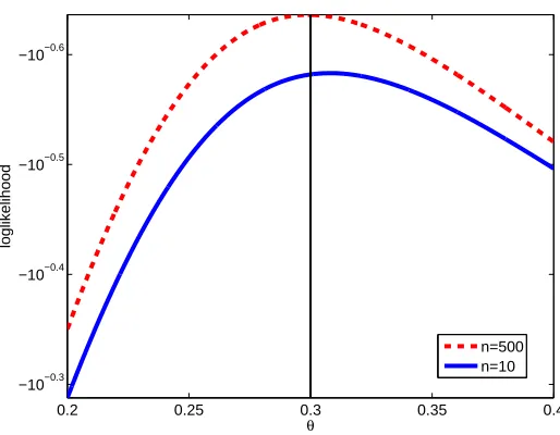
Figure 2: A plot of the loglikelihood function ℓ(θ) in the case of regression for k = 1 with

θtrue_{=0.3,τ=1, µ}

y=0 andσy=0.2. As additional unlabeled examples are added the

loglikelihood curve become steeper and their maximizers get closer to the true parameter

In the case of regression (12) involves an integral over a product of k+1 Gaussians, assuming that y_∼N(µy,σ2y). In this case the integral in (12) simplifies to

p_θ(yˆ₁(i), . . . ,yˆ(_ki)) =

Z ∞

−∞

k

∏

j=1

1

θjτ √

2πe

−yˆ(_ji)−θjy(i)

2

2θ2 jτ2

! 1

σy √

2πe

−(y(i)−µy)

2.

2σ2y_dy(i)

= 1

τk₍√₂π₎k+1σ

y∏kj=1θj

Z ∞

−∞exp  − 1 2  

y(i)₋µy

σy

!2 +

k

∑

j=1

y(i)

τ −

ˆ

y(_ji)

τθj

!2  

dy(i)

=

R∞

−∞exp

−12

1 σ2 y+ k τ2

(y(i))2₊

µy

σ2

y+∑

k j=1

ˆ y(_ji)

τ2θ j

y(i)₋1₂

µ2 y

σ2

y+∑

k j=1

(yˆ(_ji))2 τ2_θ2

j

τk₍√₂π₎k+1σ

y∏kj=1θj

=

√_πh

1 2 1 σ2 y + k τ2 i−1/2

τk₍√₂π₎k+1σ

y∏kj=1θj

exp      µy σ2

y+∑

k j=1

ˆ y(ji)

τ2_θ j 2 2 1 σ2 y+ k τ2 − k

∑

j=1

(yˆ(_ji))2

2τ2θ2 j

− µ 2 y

2σ2 y      (13)

where the last equation was obtained using Lemma 1 concerning Gaussian integrals. Note that this equation does not have a closed form maximizer requiring the use of iterative computational techniques.

2.3 Collaborative Estimation of the Risks: Conditionally Correlated Predictors

In some cases the conditional independence assumption made in the previous subsection does not hold and the factorization (12) is violated. In this section, we discuss how to relax this assumption in the classification case. A similar approach may also be used for regression. We omit the details here due to notational clarity.

There are several ways to relax the conditional independence assumption. Most popular, per-haps, is the mechanism of hierarchical loglinear models for categorical data (Bishop et al., 1975). For example, generalizing our conditional independence assumption to second-order interaction log-linear models we have

log p(yˆ1, . . . ,yˆk|y) =αy+ l

∑

i=1

βi,yˆi,y+

∑

i<j

γi,j,yˆi,yˆj,y (14)

where the following ANOVA-type parameter constraints are needed (Bishop et al., 1975)

0=

∑

ˆ yi

βi,yˆi,y ∀i,y, (15)

0=

∑

ˆ yi

γi,j,yˆi,yˆj,y=

∑

ˆ yj

γi,j,yˆi,yˆj,y ∀i,j,y.

Theβparameters in (14) correspond to the order-1 interaction between the variables ˆy1, . . . ,yˆk,

conditioned on y. They correspond to theθiin the independent formulation (6)-(8). Theγparameters

In the case of classification, the number of degrees of freedom or free unconstrained parameters in (14) depends on whether the number of classes is 2 or more and what additional assumptions exist onβandγ. For example, assuming that the probability of fi,fjmaking an error depends on the true

class y but not on the predicted classes ˆyi,yˆjresults in a k+k2parameters. Relaxing that assumption

but assuming binary classification results in 2k+4k2 parameters. The estimation and aggregation

techniques described in Section 2.1 work as before with a slight modification of replacing (6)-(8) with variations based on (14) and enforcing the constraints (15).

Equation (14) captures two-way interactions but cannot model higher order interactions. How-ever, three-way and higher order interaction models are straightforward generalizations of (14) cul-minating in the full loglinear model which does not make any assumption on the statistical

depen-dency of the noise operators T1, . . . ,Tk. However, as we weaken the assumptions underlying the

loglinear models and add higher order interactions the number of parameters increases adding to the difficulty in estimating the risks R(f1), . . . ,R(fk).

In our experiments on real world data (see Section 7), it is often the case that maximizing the loglikelihood under the conditionally independent assumption (12) provides adequate accuracy and there is no need for the more general (14)-(15). Nevertheless, we include here the case of loglinear models as it may be necessary in some situations.

3. Extensions: Missing Values, Active Learning, and Semi-Supervised Learning

In this section, we discuss extensions to the current framework. Specifically, we consider extending the framework to the cases of missing values, active and semi-supervised learning.

Occasionally, some predictors are unable to provide their output over specific data points. That is assuming a data set x(1), . . . ,x(n)each predictor may provide output on an arbitrary subset of the data points_{fj(x(i)): i∈Sj}, where Sj⊂ {1, . . . ,n}, j=1, . . . ,k.

Commonly referred to as a missing value situation, this scenario may apply in cases where dif-ferent parts of the unlabeled data are available to the difdif-ferent predictors at test time due to privacy, computational complexity, or communication cost. Another example where this scenario applies is active learning where operating fjinvolves a certain cost cj≥0 and it is not advantageous to operate

all predictors with the same frequency for the purpose of estimating the risks R(f1), . . . ,R(fk). Such

is the case when fjcorresponds to judgments obtained from human experts or expensive machinery

that is busy serving multiple clients. Active learning fits into this situation with Sj denoting the set

of selected data points for each predictor.

We proceed in this case by defining indicators βji denoting whether predictor j is available

to emit fj(x(i)). The risk estimation proceeds as before with the observed likelihood modified to

account for the missing values.

In the case of collaborative estimation with conditional independence, the estimator and log-likelihood become

ˆ

θmle

n =arg max

θ ℓ(θ),

ℓ(θ) =

n

∑

i=1

log

∑

r:βri=0

Z

Y

pθ(yˆ(₁i), . . . ,yˆ_k(i))dµ(yˆ(ri)) (16)

=

n

∑

i=1

log

∑

r:βri=0

ZZ

Y2pθ(yˆ (i)

1 , . . . ,yˆ

(i)

k |y(

i)_)p(y(i)_)dµ(yˆ(i)

where pθmay be further simplified using the non-collaborative approach, or using the collaborative approach with conditional independence or loglinear model assumptions.

In the case of semi-supervised learning a small set of labeled data is augmented by a large set of unlabeled data. In this case our framework remains as before with the likelihood summing over the observed labeled and unlabeled data. For example, in the case of collaborative estimation with conditional independence we have

ℓ(θ) =

n

∑

i=1

log Z

Y

k

∏

j=1

pθj(yˆ (i)

j |y(i))p(y(i))dµ(y(i)) + m

∑

i=n+1

log

k

∏

j=1

pθj(yˆ (i)

j |y(i))p(y(i)).

The different variations concerning missing values, active learning, semi-supervised learning, and non-collaborative or collaborative estimation with conditionally independent or correlated noise processes can all be combined in different ways to provide the appropriate likelihood function. This provides substantial modeling flexibility.

4. Consistency of ˆθmle_n and ˆR(fj)

In this and the next section we consider the statistical behavior of the estimator ˆθmle_n defined in (2) and the risk estimator ˆR(fj) =gj(θˆmle) defined in (1). The analysis is conducted under the

assumption that the vectors of observed predictors outputs ˆy(i)= (yˆ₁(i), . . . ,yˆ(_ki))are iid samples from the distribution

pθ(yˆ) =pθ(yˆ1, . . . ,yˆk) =

Z

Y

pθ(yˆ1, . . . ,yˆk|y)p(y)dµ(y).

We start by investigating whether estimator ˆθmle in (2) converges to the true parameter value. More formally, strong consistency of the estimator ˆθmle_n =θˆ(yˆ(1), . . . ,yˆ(n)), ˆy(1), . . . ,yˆ(n)_∼iid p_θ0 is

defined as strong convergence of the estimator toθ0as n→∞(Ferguson, 1996)

lim

n→∞ ˆ

θmle

n (yˆ(1), . . . ,yˆ(n)) =θ0with probability 1.

In other words as the number of samples n grows, the estimator will surely converge to the true

parameterθ0governing the data generation process.

Assuming that the risks R(fj) =gj(θ)are defined using continuous functions gj, strong

consis-tency of ˆθmle implies strong convergence of ˆR(fj)to R(fj). This is due to the fact that continuity

preserves limits. Indeed, as the gj functions are continuous in both the classification and regression

cases, strong consistency of the risk estimators ˆR(fj)reduces to strong consistency of the estimators

ˆ

θmle_.

It is well known that the maximum likelihood estimator is often strongly consistent. Consider, for example, the following theorem.

Proposition 2 (e.g., Ferguson, 1996) Let ˆy(1), . . . ,yˆ(n)_∼iid pθ0, θ0∈Θ. If the following conditions

hold

1. Θis compact (compactness)

2. p_θ(yˆ)is upper semi-continuous inθfor all ˆy (continuity)

3. There exists a function K(yˆ)such thatEpθ0|K(yˆ)|<∞ (boundedness)

and log p_θ(yˆ)₋log p_θ0(yˆ)_≤K(yˆ) _∀yˆ _∀θ

4. For allθand sufficiently smallρ>0, sup_|θ′_−θ|<ρpθ′(yˆ)is (measurability)

measurable in ˆy

then the maximum likelihood estimator is strongly consistent, that is, ˆθmle→θ0 as n→∞ with

probability 1.

Note that p_θ(yˆ) in the proposition above corresponds to R

Y pθ(yˆ|y)p(y)dµ(y) in our framework.

That is the MLE operates on the observed data or predictor output ˆy(1), . . . ,yˆ(n) that is sampled iid from the distribution p_θ0(yˆ) =

R

Y pθ0(yˆ|y)p(y)dµ(y).

Of the five conditions above, the last condition of identifiability is the only one that is truly prob-lematic. The first condition of compactness is trivially satisfied in the case of classification. In the case of regression it is satisfied assuming that the regression parameter and model parameter are fi-nite and a₆=0 as the estimator ˆθmlewill eventually lie in a compact set. The second condition of con-tinuity is trivially satisfied in both classification and regression as the functionR

Y pθ(yˆ|y)p(y)dµ(y)

is continuous inθonce ˆy is fixed. The third condition is trivially satisfied for classification (finite

valued y). In the case of regression due to conditions 1,2 (compactness and semi-continuity) we can replace the quantifier_∀θwith a particular valueθ′_∈Θrepresenting worst case situation in the bound of the logarithm difference. Then, the bound K may be realized by the difference of log

terms (with respect to that worst caseθ′) whose expectation converges to the KL divergence which

in turn is never∞for Gaussian distributions or its derivatives. The fourth condition of measurability

follows as p_θ is specified in terms of compositions, summations, multiplications, and point-wise

limits of well-known measurable functions.

The fifth condition of identifiability states that if pθ(yˆ)and pθ0(yˆ)are identical as functions, that is, they are identical for every value of ˆy, then necessarilyθ=θ0. This condition does not hold in

general and needs to be verified in each one of the special cases.

We start with establishing consistency in the case of classification where we rely on a symmetric noise model (8). The non-symmetric case (6) is more complicated and is treated afterwards. We conclude the consistency discussion with an examination of the regression case.

4.1 Consistency of Classification Risk Estimation

Proposition 3 Let f1, . . . ,fkbe classifiers fi:

X

Y

Y

processes described by (8). If the classifiers are weak learners, that is, 1/l<1₋err(fi)<1 and

p(y)is not uniform the unsupervised collaborative diagnosis model is identifiable.

Corollary 4 Let f1, . . . ,fkbe classifiers fi:

X

Y

Y

(8). If the classifiers are weak learners, that is, 1/l<1₋err(fi)<1, and p(y)is not uniform the

unsupervised non-collaborative diagnosis model is identifiable.

Proof Proving identifiability in the non-collaborative case proceeds by invoking Proposition 3

(whose proof is given below) with k=1 separately for each classifier. The conditional

indepen-dence assumption in Proposition 3 becomes redundant in this case of a single classifier, resulting in identifiability of p_θj(yˆj)for each j=1, . . . ,k

Corollary 5 Under the assumptions of Proposition 3 or Corollary 4 the unsupervised maximum

likelihood estimator is consistent, that is,

P

lim

n→∞ ˆ

θmle

n (yˆ(1), . . . ,y(n)) = (θtrue1 , . . . ,θtruek )

Consequentially, assuming that R(fj) =gj(θ),j=1, . . . ,k with continuous gj we also have

P

lim

n→∞Rˆ(fj; y

(1)_{, . . . ,y}(n)_{) =R(f}

j), ∀j=1, . . . ,k

=1.

Proof Proposition 3 or Corollary 4 establishes identifiability, which in conjunction with Proposi-tion 2 proves the corollary.

Proof (for Proposition 3) We prove identifiability by induction on k. In the base case of k=1, we have a set of l equations, corresponding to i=1,2. . .l,

pθ(yˆ1=i) = p(y=i)θ1+

∑

p(y= j) !

(1₋θ1)

(l₋1)

= p(y=i)θ1+ (1−p(y=i))

(1₋θ1)

(l−1)

= θ1(l p(y=i)−1) +1−p(y=i) (l₋1)

from which we can see that ifη₆=θand p(y=i)₆=1/l then p_θ(yˆ1)6=pη(yˆ1). This proves

identifi-ability for the base case of k=1.

Next, we assume identifiability holds for k and prove that it holds for k+1. We do so by

deriving a contradiction from the assumption that identifiability holds for k but not for k+1. We

denote the parameters corresponding to the k labelers by the vectorsθ,η_∈[0,1]k_{and the parameters}

corresponding the additional k+1 labeler byθk+1,ηk+1.

In the case of k classifiers we have

pθ(yˆ1, . . . ,yˆk) = l

∑

i=1

pθ(yˆ1, . . . ,yˆk|y=i)p(y=i) = l

∑

i=1

G(

A

where

G(

A

def

=p(y=i)

∏

j∈Ai

θj·

∏

(1₋θj)

(l₋1) ,

A

def

=_{j_{∈ {}1,2...,k_}: ˆyj=i}.

Note that the

A

A

In order to have unidentifiability for the k+1 classifiers we need(θ,θk+1)6= (η,ηk+1)and the

corre-sponds to any partition

A

A

θk+1G(

A

(1₋θk+1)

(l₋1) _i

∑

A

A

(1₋ηk+1)

(l₋1) _i

∑

A

θk+1G(

A

(1₋θk+1)

(l₋1) _i

∑

A

A

(1₋ηk+1)

(l₋1) _i

∑

A

.

θk+1G(

A

(1₋θk+1)

(l₋1)

∑

A

A

(1₋ηk+1)

(l₋1)

∑

A

We consider two cases in which(θ,θk+1)6= (η,ηk+1): (a) θ6=η, and (b)θ=η,θk+16=ηk+1.

In the case of (a) we add the l equations above which marginalizes ˆyk+1 out of pθ(yˆ1, . . . ,yˆk,yˆk+1)

and p_η(yˆ1, . . . ,yˆk,yˆk+1)to provide l

∑

i=1

G(

A

l

∑

i=1

G(

A

which together withθ₆=ηcontradicts the identifiability for the case of k classifiers. In case (b) we have from the l equations above

θk+1G(

A

1₋θk+1

l−1

l

∑

i=1

G(

A

A

=ηk+1G(

A

1₋ηk+1

l₋1

l

∑

i=1

G(

A

A

for any t_{∈ {}1, . . . ,l_}which simplifies to

0= (θk+1−ηk+1) lG(

A

∑

i=1

G(

A

!

t=1, . . . ,k.

As we assume at this point thatθk+16=ηk+1the above equality entails

lG(

A

∑

i=1

G(

A

We show that (17) cannot hold by examining separately the cases p(y=t)>1/l and p(y=t)<1/l.

Recall that there exists a t for which p(y=t)₆=1/l since the proposition requires that p(y)is not uniform.

If p(y=t)>1/l we choose

A

l p(y=t)

k

∏

j=1

θj=

∑

p(y=i)

k

∏

j=1

1₋θj

l₋1 +p(y=t)

k

∏

j=1 θj

(l₋1)p(y=t)

k

∏

j=1

θj= (1−p(y=t)) k

∏

j=1

1₋θj

l₋1

p(y=t)

k

∏

j=1 θj=

(1₋p(y=t)) (l−1)

k

∏

j=1

1₋θj

which cannot hold as the term on the left hand side is necessarily larger than the term on the right hand side (if p(y=t)>1/l andθj >1/l). In the case p(y=t)<1/l we choose

A

s₆=t to obtain

l p(y=t)

k

∏

j=1

1₋θj

l₋1 =_i

∑

k

∏

j=1

1₋θj

l₋1 +p(y=s)

k

∏

j=1 θj

(l p(y=t)₋p(y₆=s))

k

∏

j=1

1₋θj

l₋1 =p(y=s)

k

∏

j=1 θj

which cannot hold as the term on the left hand side is necessarily smaller than the term on the right hand side (if p(y=t)<1/l andθj>1/l).

Since we derived a contradiction to the fact that we have k-identifiability but not k+1 identifia-bility, the induction step is proven which establishes identifiability for any k_≥1.

The conditions asserted above that p(y)₆=1/l and 1/l<1₋err(fi)<1 are intuitive. If they

are violated a certain symmetry may emerge which renders the model non-identifiable and the MLE estimator not consistent.

In the case of the non-collaborative estimation for binary classification with the non-symmetric

noise model, the matrixθin (6) is a 2_×2 matrix with two degrees of freedom as each row sums to

one. In particular we haveθ11=pθ(yˆ=1|y=1),θ12=pθ(yˆ=1|y=2), θ21=pθ(yˆ=2|y=1), θ22=pθ(yˆ=2|y=2)with the overall risk R(f) =1−θ11p(y=1)−θ22p(y=2). Unfortunately, the

matrixθis not identifiable in this case and neither is the scalar parameterθ11p(y=1) +θ22p(y=2)

that can be used to characterize the risk.

We can, however, obtain a consistent estimator forθ(and therefore for R(f)) by first showing that the parameterθ11p(y=1)−θ22p(y=2)is identifiable and then taking the intersection of two

such estimators.

Lemma 6 In the case of the collaborative estimation for binary classification with the

non-symmetric noise model and p(y)₆=0, the parameterθ11p(y=1)−θ22p(y=2)is identifiable.

Proof For two different parameterizationsθ,ηwe have

pθ(yˆ=1) =p(y=1)θ11+ (1−p(y=1))(1−θ22), (18)

pθ(yˆ=2) =p(y=1)(1−θ11) + (1−p(y=1))θ22 (19)

and

p_η(yˆ=1) =p(y=1)η11+ (1−p(y=1))(1−η22), (20)

pη(yˆ=2) =p(y=1)(1₋η11) + (1−p(y=1))η22. (21)

Equating the two Equations (18) and (20) we have

p(y=1)(θ11+θ22) +1−p(y=1)−θ22=p(y=1)(η11+η22) +1−p(y=1)−η22

p(y=1)θ11−(1−p(y=1))θ22=p(y=1)η11−(1−p(y=1))η22

Similarly, equating Equation (19) and Equation (21) also results in p(y=1)θ11−p(y=2)θ22=

p(y=1)η11−p(y=2)η22. As a result, we have

p_θ≡p_{η ⇒} p(y=1)θ11−p(y=2)θ22=p(y=1)η11−p(y=2)η22.

The above lemma indicates that we can use the maximum likelihood method to obtain a consis-tent estimator for the parameterθ11p(y=1)−θ22p(y=2). Unfortunately the parameterθ11p(y=

1)₋θ22p(y=2)does not have a clear probabilistic interpretation and does not directly characterize

the risk. As the following proposition shows we can obtain a consistent estimator for the risk R(f) if we have two populations of unlabeled data drawn from distributions with two distinct marginals

p1(y)and p2(y).

Proposition 7 Consider the case of the non-collaborative estimation of binary classification risk

with the non-symmetric noise model. If we have access to two unlabeled data sets drawn indepen-dently from two distributions with different marginals, that is,

x(1), . . . ,x(n)∼iid p1(x) =

∑

p(x|y)p1(y),

x′(1), . . . ,x′(m)_∼iid p2(x) =

∑

p(x_|y)p2(y)

we can obtain a consistent estimator for the classification risk R(f).

Proof Operating the classifier f on both sets of unlabeled data we get two sets of observed clas-sifier outputs ˆy(1)_{, . . . ,yˆ}(n)_{, ˆy}′(1)_{, . . . ,yˆ}′(m)_{where ˆy}(i) iid

∼∑ypθ(yˆ|y)p1(y)and ˆy′(i)

iid

∼∑ypθ(yˆ|y)p2(y).

In particular, note that the marginal distributions p1(y) and p2(y) are different but the parameter

matrixθis the same in both cases as we operate the same classifier on samples from the same class

conditional distribution p(x_|y).

Based on Lemma 6 we construct a consistent estimator for p1(y=1)θ11−p1(y=2)θ22 by

maximizing the likelihood of ˆy(1), . . . ,yˆ(n). Similarly, we construct a consistent estimator for p2(y=

1)θ11−p2(y=2)θ22 by maximizing the likelihood of ˆy′(1), . . . ,yˆ′(m). Note that p1(y=1)θ11−

p1(y=2)θ22and p2(y=1)θ11−p2(y=2)θ22describe two lines in the 2-D space(θ11,θ22). Since

the true value ofθ11,θ22 represent a point in that 2-D space belonging to both lines, it is

neces-sarily the intersection of both lines (the lines cannot be parallel since their linear coefficients are distributions which are assumed to be different).

As n and m increase to infinity, the two estimators converge to the true parameter values. As a result, the intersection of the two lines described by the two estimators converges to the true values of(θ11,θ22)thus allowing reconstruction of the matrixθand the risk R(f).

Clearly, the conditions for consistency in the asymmetric case are more restricted than in the symmetric case. However, situations such as in Proposition 7 are not necessarily unrealistic. In many cases it is possible to identify two unlabeled sets with different distributions. For example, if

hospitals or two different regions with different marginal distribution corresponding to the frequency of the medical condition.

As indicated in the previous section, the risk estimation framework may be extended beyond non-collaborative estimation and collaborative conditionally independent estimation. In these ex-tensions, the conditions for identifiability need to be determined separately, in a similar way to Corollary 4. A systematic way to do so may be obtained by noting that the identifiability equations

0=p_θ(yˆ1, . . . ,yˆk)−pη(yˆ1, . . . ,yˆk) ∀yˆ1, . . . ,yˆk

is a system of polynomial equations in (θ,η). As a result, demonstrating lack of identifiability becomes equivalent to obtaining a solution to a system of polynomial equations. Using Hilbert’s Nullstellensatz theorem we have that a solution to a polynomial system exists if the polynomial system defines a proper ideal of the ring of polynomials (Cox et al., 2006). As k increases the

chance of identifiability failing decays dramatically as we have a system of lk polynomials with 2k

variables. Such an over-determined system with substantially more equations than variables is very unlikely to have a solution.

These observations serve as both an interesting theoretical connection to algebraic geometry as well as a practical tool due to the substantial research in computational algebraic geometry. See Sturmfels (2002) for a survey of computational algorithms and software associated with systems of polynomial equations.

4.2 Consistency of Regression Risk Estimation

In this section, we prove the consistency of the maximum likelihood estimator ˆθmlein the regression case. As in the classification case our proof centers on establishing identifiability.

Proposition 8 Let f1, . . . ,fkbe regression models fi(x) =a′ix with y∼N(µy,σ2y), y=ax+ε.

Assum-ing that a₆=0 the unsupervised collaborative estimation model assuming conditionally independent

noise processes (12) is identifiable.

Corollary 9 Let f1, . . . ,fkbe regression models fi(x) =a′ix with y∼N(µy,σ2y), y=ax+ε. Assuming

that a₆=0 the unsupervised non-collaborative estimation model (12) is identifiable.

Proof Proving identifiability in the non-collaborative case proceeds by invoking Proposition 8

(whose proof is given below) with k=1 separately for each regression model. The conditional

independence assumption in Proposition 8 becomes redundant in this case of a single predictor, re-sulting in identifiability of p_θj(yˆj)for each j=1, . . . ,k.

Corollary 10 Under the assumptions of Proposition 8 or Corollary 9 the unsupervised maximum

likelihood estimator is consistent, that is,

P

lim

n→∞ ˆ

θmle

n (yˆ(1), . . . ,y(n)) = (θtrue1 , . . . ,θtruek )

=1.

Consequentially, assuming that R(fj) =gj(θ),j=1, . . . ,k with continuous gj we also have

P

lim

n_→∞

ˆ

R(fj; y(1), . . . ,y(n)) =R(fj), ∀j=1, . . . ,k

Proof Proposition 8 or Corollary 9 establish identifiability, which in conjunction with Proposition 2 completes the proof.

Proof (of Proposition 8).

We will proceed, as in the case of classification, with induction on the number of predictors k. In the base case of k=1 we have derived pθ1(yˆ1)in Equation (11). Substituting in it ˆy1=0 we get

P_θ1(yˆ1=0) =

1

θ1

q

2π(τ2₊σ2 y)

exp µ

2 y

2σ2 y

τ2 σ2

y+τ2 −1

!!

,

P_η1(yˆ1=0) =

1

η1

q

2π(τ2₊σ2 y)

exp µ

2 y

2σ2 y

τ2 σ2

y+τ2−

1 !!

.

The above expression leads toθ16=η1⇒pθ1(yˆ1=0)6=pη1(yˆ1=0)which implies identifiability. In the induction step we assume identifiability holds for k and we prove that it holds also for k+1 by deriving a contradiction to the assumption that it does not hold. We assume that identifiability fails in the case of k+1 due to differing parameter values, that is,

p(θ,θk+1)(yˆ1, . . . ,yˆk,yˆk+1) =p(η,ηk+1)(yˆ1, . . . ,yˆk,yˆk+1)∀yˆj∈R j=1, . . . ,k+1 (22) with(θ,θk+1)6= (η,ηk+1)whereθ,η∈Rk. There are two cases which we consider separately: (a) θ6=ηand (b)θ=η.

In case (a) we marginalize both sides of (22) with respect to ˆyk+1which leads to a contradiction

to our assumption that identifiability holds for k

Z ∞

−∞

p_(θ,θk+1)(yˆ1, . . . ,yˆk,yˆk+1)d ˆyk+1=

Z ∞

−∞

p_(η,ηk+1)(yˆ1, . . . ,yˆk,yˆk+1)d ˆyk+1

pθ(yˆ1, . . . ,yˆk) =pη(yˆ1, . . . ,yˆk).

In case (b) θ=ηandθk+16=ηk+1. Substituting ˆy1=···=yˆk+1 =0 in (22) (see (13) for a

derivation) we have

P(θ,θk+1)(yˆ1=0, . . . ,yˆk+1=0) =P(η,ηk+1)(yˆ1=0, . . . ,yˆk+1=0) or

√_πh

1 2 1 σ2 y +

k+1

τ2

i−1/2

τk+1₍√₂π₎k+2σ

yθk+1∏kj=1θj

exp    _µ y σ2 y 2 2 1 σ2 y+

k+1

τ2

−

µ2_y

2σ2 y



 

=

√_πh

1 2 1 σ2 y+

k+1

τ2

i−1/2

τk+1₍√₂π₎k+2σ

yηk+1∏kj=1ηj

exp    _µ y σ2 y 2 2 1 σ2 y+

k+1

τ2

−

µ2_y

2σ2 y



 

5. Asymptotic Variance of ˆθmle_n and ˆR

A standard result from statistics is that the MLE has an asymptotically normal distribution with mean vector θtrue and variance matrix (nJ(θtrue₎₎−1_{, where J(θ) is the r×r Fisher information}

matrix

J(θ) =Epθ{∇log pθ(yˆ)(∇log pθ(yˆ))⊤}

with ∇log p_θ(yˆ) represents the r_×1 gradient vector of log p_θ(yˆ) with respect toθ. Stated more

formally, we have the following convergence in distribution as n_→∞(Ferguson, 1996)

√

n(_θˆmle

n −θ0) N(0,J−1(θtrue)). (23)

It is instructive to consider the dependency of the Fisher information matrix, which corresponds to the asymptotic estimation accuracy, on n,k,p(y),θtrue_.

In the case of classification considering (8) with k=1 and

Y

J(θ) = α(2α−1)

2

(θ(2α₋1)₋α+1)2−

(2α₋1)2_(α−1)

(α₋θ(2α₋1))2 (24)

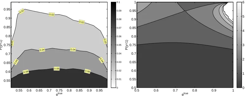
whereα=P(y=1). As Figure 3 (right) demonstrates, the asymptotic accuracy of the MLE (as

indicated by J) tends to increase with the degree of non-uniformity of p(y). Recall that since identi-fiability fails for a uniform p(y)the risk estimate under a uniform p(y)is not consistent. The above derivation (24) is a quantification of that fact reflecting the added difficulty in estimating the risk as

we move closer to a uniform label distributionα_→1/2. The dependency of the asymptotic

accu-racy onθtrue_{is more complex, tending to favor}θtrue_{values close to 1 or 0.5. Figure 3 (left) displays}

the empirical accuracy of the estimator as a function of p(y)andθtrueand shows remarkable simi-larity to the contours of the Fisher information (see Section 7 for more details on the experiments). In particular, whenever the estimation error is high the asymptotic variance of the estimator is high (or equivalently, the Fisher information is low). For instance, the top contours in the left panel have smaller estimation error on the top right than in the top left. Similarly, the top contours in the right panel have smaller asymptotic variance on the top right than on the top left. We thus conclude that the Fisher information provides practical, as well as theoretical insight into the estimation accuracy. Similar calculations of J(θtrue_{) for collaborative classification case or for the regression case}

result in more complicated but straightforward derivations. It is important to realize that consistency is ensured for any identifiable θtrue,p(y). The value(J(θtrue₎₎−1 _{is the constant dominating that}

consistency convergence.

A similar distributional analysis can be derived for the risk estimator. Applying Cramer’s theo-rem (Ferguson, 1996) to ˆR(fj) =gj(θˆmle), j=1, . . . ,k and (23) we have

√

n(_Rˆ_{(f)−R(f)) N0,∇g(θ}true_)J(θtrue_)∇g(θtrue₎⊤

where R(f),_Rˆ_{(f)are the vectors of true risk and risk estimates for the different predictors f1, . . . ,fk} and∇g(θtrue_{)is the Jacobian matrix of the mapping g= (g1, . . . ,g}

k)evaluated atθtrue.

For example, in the case of classification with k=1 we have R(fj) =1−θj and the Jacobian

matrix is₋1, leading to an identical asymptotic distribution to that of the MLE (23)-(24)

√

n(Rˆ(f)₋R(f)) N 0,

α

(2α₋1)2

(θ(2α₋1)₋α+1)2−

(2α₋1)2₍α₋₁₎

(α₋θ(2α₋1))2

−1!

6. Optimization Algorithms

Recall that we obtained closed forms for the likelihood maximizers in the cases of non-collaborative estimation for binary classifiers and non-collaborative estimation for one dimensional regression models. The lack of closed form maximizers in the other cases necessitates iterative optimization techniques.

One class of technique for optimizing nonlinear loglikelihoods is the class of gradient based methods such as gradient descent, conjugate gradients, and quasi Newton methods. These tech-niques proceed iteratively following a search direction; they often have good performance and are easy to derive. The main difficulty with their implementation is the derivation of the loglikelihood and its derivatives. For example, in the case of collaborative estimation of classification (l_≥2) with symmetric noise model and missing values the loglikelihood gradient is

∂ℓ ∂θj

=

n

∑

i=1 ∑

y(i)

p(y(i)) ∑

r:βri=0 ∑ ˆ y(ri)

∏p6=jhpi(I(yˆ(_ji)=y(i))−θj)((l−1)θj)I(yˆ

(i)

j =y(i))−1₍₁₋θ

j)−I(yˆ

(i)

j =y(i))

∑y(i)p(y(i))∑_r:β_ri=0∑

ˆ y(ri)∏

k p=1hpi

,

hpi=θ

I(yˆ(pi)=y(i))

p

1₋θp

l−1

I(yˆ(pi)6=y(i))

Similar derivations may be obtained in the other cases in a straightforward manner.

An alternative iterative optimization technique for finding the MLE is expectation maximization (EM). The derivation of the EM update equations is again relatively straightforward. For example

in the above case of collaborative estimation of classification (l_≥2) with symmetric noise model

and missing values the EM update equations are

θ(t+1)_{=arg max}

θ

n

∑

i=1

∑

∑

∑

ˆ y(ri)

q(t)(yˆr(i),y(i)) k

∑

j=1

log pj(yˆ(ji)|y( i)₎

=1

n

n

∑

i=1

∑

∑

∑

ˆ y(ri)

q(t)(yˆ(ri),y(i))I(yˆ(ji)=y(i)),

q(t)(yˆr(i),y(i)) =

p(y(i))∏k

j=1pj(yˆ( i)

j |y(i),θ(t))

∑y(i)∑_r:β_ri=0∑

ˆ y(ri)p(y

(i)_)∏k

j=1pj(yˆ(ji)|y(i),θ(t)) .

where q(t)is the conditional distribution defining the EM bound over the loglikelihood function. If all the classifiers are always observed, that is,βri=1∀r,i Equation (16) reverts to (12), and

the loglikelihood and its gradient may be efficiently computed in O(nlk2). In the case of missing classifier outputs a naive computation of the gradient or EM step is exponential in the number of

missing values R=maxi∑rβri. This, however, can be improved by careful dynamic programming.

For example, the nested summations over the unobserved values in the gradient may be computed using a variation of the elimination algorithm in O(nlk2R)time.

7. Empirical Evaluation