Scalable Correlated Sampling for Join Query Estimations on Big Data

Volume 64, 2019, Pages 41–50

Proceedings of 28th International Conference on Software Engineering and Data Engineering

Scalable Correlated Sampling for Join Query Estimations

on Big Data

David S. Wilson

, Wen-Chi Hou

, and Feng Yu

1 _{Youngstown State University, Youngstown, OH, USA}

[email protected],[email protected] 2

Southern Illinois Univeristy, Carbondale, IL, USA [email protected]

Abstract

Estimate query results within limited time constraints is a challenging problem in the research of big data management. Query estimation based on simple random samples per-forms well for simple selection queries; however, return results with extremely high relative errors for complex join queries. Existing methods only work well with foreign key joins, and the sample size can grow dramatically as the dataset gets larger. This research imple-ments a scalable sampling scheme in a big data environment, namely correlated sampling in map-reduce, that can speed up search query length results, give precise join query esti-mations, and minimize storage costs when presented with big data. Extensive experiments with large TPC-H datasets in Apache Hive show that our sampling method produces fast and accurate query estimations on big data.

1

Introduction

Big data is everywhere. Approximately 2.5 quintillion bytes (2.5 billion Gigabytes) of data is produced each day. Ninety percent of the data created in the world has been created in the past two years [9]. To put that into perspective, IBM created the IBM Model 350 Disk File in 1956. It was the size of a compact-size car, and had a storage capacity of five megabytes. If one were to place these machines side by side, based off the amount of data we use in one day, they would circle the earth nine thousand one hundred and ninety times. With the sizes of company databases reaching terabytes and even petabytes, and at the speed of which this data is being accumulated, the need for query optimization has never been so high.

The rest of this work is organized as follows. Section2states the background of the problem. Correlated sampling on big data is elaborated in section3. Experiment results are presented in section4. Section5concludes the work.

2

Background

2.1

Big Data Management

Big Data may just be one of the most misunderstood terms in the technology field. It is miscommonly referred to as a large volume of data. While not entirely incorrect, there is much more to Big Data then just size. In the following sections, the origins of big data, as well as what defines data as “Big data”, will be discussed.

The term “Big Data” was first coined in 1998 by John Mashey of Silicon Graphics, Inc., al-though this is debated [13]. Others had written about big data before this date, but Mr.Mashey was the first that used the term in the context of computing. Even though the term Big Data was created in the 90’s it was not until the early 2000’s that it took the form of what is is considered today. In February 2001, Doug Laney created the three V’s of Big Data, which are Volume, Variety, and Velocity. [6]

The Apache Hadoop framework [15] consists of multiple modules, each having its own dis-tinctive responsibilities. Hadoop Common is the storehouse for other Hadoop Modules. It holds all of the files in which the other Hadoop Modules need to run properly. Hadoop Distributed File System, or HDFS for short,[2] deals with the storage of data of a Hadoop cluster. A major issue with storing streaming, large sets of data, is hardware failure. HDFS is built to combat this, by using a process called replication. HDFS consists of a name node, which stores all meta data of all files stored. It also has data nodes as well, which hold all of the actual data. Each data node consists of a multitude of blocks, with each block of data being stored into 3 different data node locations in the cluster. If at any time there is a node that fails, or a machine in the cluster fails, another block copy is made on another node or machine.

2.2

Database Systems on Big Data

With the rise of big data, many database systems have been developed on big data for scalable data management and processing such as Hive[12], HBase[14], Dynamo[5], etc. Among them, Hive was created to make it easier for users to be able to use Hadoop’s Map-Reduce and HDFS without an advanced knowledge of Java. As mentioned earlier, Hive uses a similar language to SQL, called HQL or Hive Query Language. With the use of this language users are able to perform data queries, as well as summarize and analyze data. Users can use traditional command line to work in Hive, or us HWI (Hive Web Interface). HWI is a graphical user interface, or GUI, that simplifies the use of hive.

2.3

Join Graph of a Database

Definition 1. (Join Graph) A join graph [11] is a visual representation of a database in which

R2 R4

R3 R5

R1

Figure 1: A Basic Join Graph

Definition 2. (Joinable Relations) Two relations considered joinable,Ri andRk,i6=k, when

there is a path with length≥1 between the relationsRi andRk [16].

Definition 3. (Joinable Tuples) Under the assumption thatRi andRk is a joinable relation,

a tuple inRi,denoted by ti, and a tuple inRk, denotedtk, is considered joinable ifti can find a matchti+1 inRi+1,ti+1 can find a matchti+2 inRi+2, andtk−1 can find a matchtk in Rk

[16].

Figure 1 is a basic join graph of a database. It shows that Relation 1 denoted as R1, has joinable attributes with Relation 2, as well as Relation 3, denoted withR2andR3respectively.

R2 has joinable attributes with Relation 4, denoted withR4, but does not have any joinable attributes withR3or Relation 5, denoted withR5. R3has joinable attributes withR5, but no joinable attributes withR2 orR4.

2.4

Random Sampling

Random sampling has been widely adopted for query size estimations. Simple Random Sample Without Replacement, or SRSWOR, [7, 10] has previously been tested as a random sample synopsis. A SRSWOR of each relation is taken separately, and then the resulting independent samples are joined. Unfortunately, the final results end in massive errors of the join size estima-tion [3]. SRSWOR is beneficial if one is only seeking to get a size estimation on an individual relation.

2.5

Join Synopses

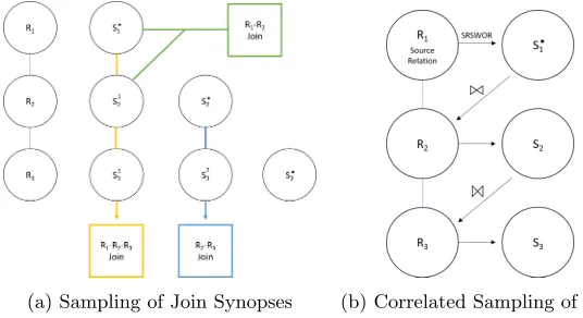
While Join Synopses (or JS) [1] use SRSWOR in its mechanics, the process does adds a join correlation between individual relations, causing a much better relative error. JS uses foreign key joins and computes samples of a small set of joins, procuring samples of all possible joins in a schema. These samples are then stored, and joined with individual SRSWOR relations to form a unbiased finalized set of correlated random tuples that can be used for query estimation. A major draw back this approach is it is quite time consuming in the sampling process. JS requires a SRSWOR on each relation in the database followed by correlated sampling on each joinable relation along the path in the join graph. For a path in a join graph consists of n

relations starting fromR1 toRn,O(n2_{) sampling operations have to be performed to generate}

(a) Sampling of Join Synopses (b) Correlated Sampling of CS2

Figure 2: Join Synopses and Correlated Sampling

3

Correlated Sampling on Big Data

3.1

Correlated Sample Synopsis

To mitigate the sampling costs of JS, Yu et al. proposed Correlated Sample Synopsis (or CS2) [16] which is a statistical summary for a database and can be used for both query estimation and approximate query processing (AQP). The purpose of CS2 is to create a unbiased, fast, and precise estimation for queries with all types of joins and selections. CS2 preserves join relationships between tuples and their relations. Unlike JS, CS2 doesn’t require SRSWOR on every relation in the join graph but employs a special value called Join Ratio (or JR) with a Reverse Estimator (or RV Estimator) to provide unbiased join query estimations.

Figure2billustrates a sample example of the process that transpires once the source relation and path selection are decided on. A simple random sample without replacement is performed on the source relation denoted as R1, with results of this SRSWOR being placed in a sample relation, denoted asS₁∗with a star to signify it is a SRSWOR ofR1. The next relation, denoted

R2is now ready to be moved to. To create the correlation between relations and preserve the join relationships,S₁∗is joined withR2, with the results being placed into a second sample relation, denoted asS2. In this example, the source relation only consists of one edge to another relation. In the case that there are multiple edges to multiple relations, one would exhaust all possibilities by creating sample relations for each relation until all edges are accounted for. Relation three, denoted asR3, is then joined withS2with the results being placed in the third sample relation, denoted asS3. The combination of all of the sample relations is considered the CS2 synopsis.

3.2

Sampling in Map-Reduce

denoted byRmap./ S. However, if both relation tables are too large to be fit into memory heaps, then a common map-reduce procedure will be initiated to compute the join result, calledreduce join, denoted byRreduce./ S. Given the same data, reduce join is more resource and time consuming compared to map join. To mitigate the sampling cost, correlated sampling on big data aims to control the sample size small enough and use map join as much as possible during the process.

3.3

Join Graph Path Creation and Source Relation Selection

Correlated Sampling begins with the creation of a join graph of the database, as well as the determined size preferred for the sample relations. A source relation selection must then be made.

It is important to note, CS2 does work with any join relationship (one-to-many, many-to-one, many-to-many). However, when selecting your sampling path and source relation it is suggested to use and follow a one relationship, as using a one-to-many or many-to-many relationship can cause the synopsis to grow considerably, subtracting from the overall number of sample tuples that can be taken from the source relation. For a complicated join graph, multiple source relations are allowed to follow many-to-one-relationships.

3.4

Correlated Sampling in Map-Reduce

Algorithm 1:Correlated Sampling in Map-Reduce

Input: G— Join Graph of the Database;na — Sample Size

forRa ∈Source Relations(G)do Sa =,Si= (∀i6=a)

Sa=Map-Reduce(SRSWOR(Ra,na))//simple random sampling onRa W ={Ra}//mark relation as visited

while ∃unvisited edge hRi, Rjiwith Ri∈W do

Sj=ΠRj(Si

map

./ Rj)//sample the next relation

W =W ∪ {Rj} //markRj as visited

end

S=Reduce({Sa} ∪ {∪j6=aSj})

end

returnS — Generated CS2 in Map-Reduce

Algorithm 1 shows the process of correlated sampling in map-reduce. For a complicated join graph, multiple source relations are allowed and the join graph can be partitioned into multiple join graph paths. For each source relation Ra in a join graph path, a SRSWOR is first performed by a map function with a small number of na tuples sampled from Ra. To

retain the joinable relations, the correlated tuples are collected in Rj when map joined with Si, which is the parent joinable relation along the join path. Note that, the join graph path

in CS2 are recommended to follow many-to-one relationships; therefore, the size of Sj is no

larger thanSi and the map join can be continued along the join path since the sample size will

generally decrease. Finally, a reduce function is initiated to collect all sampled relations intoS

3.5

Query Estimation

The process of query estimation is taking the results from a sample query, and using said results to estimate query result sizes.

3.5.1 Source Query Estimation

Source Query Estimation, is the process of estimating query results using sample queries that includes the source relation. Referring back to Figure2b, a source query would be considered a join of relationsS₁∗and S2, or a join between relationsS∗₁ andS3. The results of these joins could then be used to estimate the join query size of joins betweenR1, andR2, as well asR1

andR3.

Given S₁∗, a SRSWOR of the source relation R1 the estimation of the query result is esti-mated by

b

Ysource=N1

n1 n1

X

i=1

yi (1)

whereN1=|R1|andn1=|S1|, andyiis the number of result tuples generated by theith tuple inS₁∗.

3.5.2 No-Source Query Estimation

No-Source Query Estimation, is the process of estimating query results using sample queries that do not include the source relation. In Figure2b, a join ofS2 andS3 would be considered a No-Source Query. Due to the conditions of a No-Source query not containing a SRSWOR based off the source relation, additional steps must be taken for accurate estimation. Joinable Tuple Sampled Ratio, or JR, is a procedure of backtracking to the source relation in a no-source query (reverse sampling), and supplying it with the ability to estimate the join query size.

Given Rh the top relation in the given query and Sh the correlated sample of Rh, the estimation of the query result is estimated by

b

Yno source=N1

n1 nh

X

j=1

rjyj (2)

wherenh =|Sh|, yj is the number of result tuples generated by the jth tuple inSh, andrj is the JR value associated with thejth tuple inSh. The JR value ofrj associated with a tupleti

inRhequals the total number of joinable tuples in S1 divided by the total number of joinable tuples inR1[16].

4

Experiments

4.1

Experiment Setup

A cluster of five nodes on a remote server were created in the Sarah Cloud created in YSU Data Lab1_{. This cluster consists of two master nodes and three worker nodes. Master Node One has}

four Intel Xeon CPU’s (E5-2630 v4 @ 2.20 GHz) and 16GB of RAM. Master Node Two has two Intel Xeon CPU’s (E5-2630 v4 @ 2.20 GHz) and 10GB of RAM. All worker nodes consist

lineitem

partsupp orders

supplier

part customer

nation

region

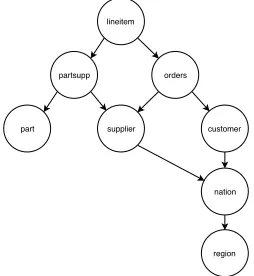
Figure 3: Sampling Graph of the TPC-H Dataset

of the same setup, a Intel Xeon CPU (E5-2630 v4 @ 2.20 GHz) processor and 8GB of RAM. The cluster is running Hadoop with Hive setup.

Two datasets are used, both datasets are generated using TPC-H benchmark[4]. The first dataset created has a total size of 1GB. The second dataset created has a total size of 10GB. Each dataset holds eight relations. The relations are Lineitem, Customer, Orders, Partsupp, Part, Supplier, Nation, and Region.

The following steps are taken to prepare for experimentation on the big data.

Step 1. Using the source dataset, a source relation as well as a join graph path must be decided on. Lineitem table holds the most many-to-one relationships, and is selected as the source relations. The sampling path that was chosen based on relationships was as follows:

Lineitem → Orders, Lineitem → Partsupp, Orders → Customer, Partsupp → Part,

Partsupp → Supplier, Customer → Nation, Nation → Region

Step 2. A empty set must be created to store the samples of the source dataset. The 1GB and 10GB datasets were denoted as tpch1g and tpch10g respectively. The sample datasets were denoted as stpch1gand s tpch10grespectively.

Step 3. Before creating the SRSWOR a sample dataset size must be selected. The decision was made that the sample dataset size would be one percent of the source dataset. The HQL to create the SRSWOR is as follows:

create table s_tpch10g.lineitem as

select * from tpch10g.lineitem where rand () <= 0.01 distribute by rand () sort by rand ();

The HQL lines distribute by rand (), and sort by rand () were added to create a higher rate of randomness. distribute by rand ()takes the entire set of tuples from a table, and distributes them randomly to different reducers. sort by rand ()then takes these sets of random tuples and sorts them randomly on each reducer.

Step 4. Using the created SRSWOR, and following the join graph path, the rest of the sample relations are constructed.

4.2

Results

Table 1: Query Search Times

Dataset Type Average (sec) Average

Speedup (1.0x) High (sec) Low (sec)

1GB source 16.26 3.05 23.24 11.57

sample 5.33 7.81 3.71

10GB source 437.49 45.91 1692.87 69.57

sample 9.53 14.84 7

“source” on all graphs, and the correlated sample dataset, is denoted as “sample”. Discussion about the results for the 1GB dataset will be presented first, followed by the 10GB dataset results, and finishing with discoveries made through the testing phase. The datasets were tested on speed of queries, as well as accuracy of the estimations.

For accuracy tests, we compare the estimated query results by CS2 (Qestimated) with the

ground truth query results from the source database (Qground truth) and calculate the absolute

relative error. The formula of the absolute relative error is given by:

Absolute Relative Error =

Qground truth−Qestimated Qground truth

×100%

1GB Experiments. Depicted in Figure 4, the 1GB dataset source dataset tests averaged a

total query time of 16.26 seconds, with a high average of 23.24 seconds in Query 11, and a low average of 11.57 seconds in Query 10. The 1GB sample dataset tests averaged 5.33 seconds, with a high average of 7.81 on Query 12, and a low average of 3.71 on Query 14. The average speed up from the sample, over the source would be a 205%. The largest speed up was Query 14 at 321.71%, and the lowest speed up was Query 9 at 141.65%. The results were impressive on the 1GB dataset with the sample dataset processing much faster than the source.

The average count of tuples for the source dataset was 2,520,952. The average count of tuples for the sample dataset was 25,385. The average join estimation results based off source join estimation was 2,538,533. The average Relative Error for the 1GB dataset was .96%. The highest relative error was 2.50% on Query 3 with the source dataset holding 592,794 tuples, the sample dataset holding 6076 tuples and source join estimation showing 607,600 tuples. The lowest relative error was .09% on query 7, with the source dataset showing 24,877, the sample dataset showing 249, and the source join estimation showing 24,900.

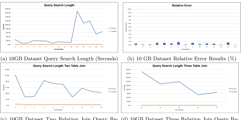
10GB Experiments. Depicted in Figure5, the 10GB dataset source dataset tests averaged a

total query time of 437.49 seconds, with a high average of 1692.87 seconds in Query 11, and a low average of 69.57 seconds in Query 7. The 1GB sample dataset tests averaged 9.53 seconds, with a high average of 14.84 on Query 11, and a low average of 7 on Query 3. The average speed up from the sample, over the source would be a 4489.44%. The largest speed up was Query 11 at 16,071.90%, and the lowest speed up was Query 2 at 758.39%. This shows that the larger the dataset, the better CS2 performs in speed.

(a) 1GB Dataset Query Search Length Results (Seconds)

(b) 1GB Dataset Relative Error Results (%)

Figure 4: Experiments of 1GB Dataset

(a) 10GB Dataset Query Search Length (Seconds) (b) 10 GB Dataset Relative Error Results (%)

(c) 10GB Dataset Two Relation Join Query Re-sults (Seconds)

(d) 10GB Dataset Three Relation Join Query Re-sults (Seconds)

Figure 5: Experiments on 10GB Dataset

The advantage of CS2 in map-reduce was recognized. Not only does CS2 speed up the join queries, but when moving from a two relation join, to a three relation join, the time increase is very minimal for CS2. In Figure5c, the two relation join query results, CS2 holds at about a seven second average while the source averages around 180 seconds. When the queries switched to a three relation join in Figure5d, the average for CS2 bumps up to about 10 seconds, while the source relation explodes and averages about 1100 seconds per query.

5

Conclusion and Future Works

to be successful in query optimization and more efficient in regards to scalability and accuracy requirements. Future research will seek to efficiently calculate JR in map-reduce proving that CS2 excel with approximate query processing in big data.

6

Acknowledgement

This research is partially supported by Cushwa Shearing Graduate Fellowship, University Re-search Council Grant, and ReRe-search Professorship Award at Youngstown State University, and Amazon Research and Education Grant.

References

[1] Swarup Acharya, Phillip B. Gibbons, Viswanath Poosala, and Sridhar Ramaswamy. Join synopses for approximate query answering. SIGMOD Rec., 28(2):275–286, June 1999.

[2] Dhruba Borthakur. The hadoop distributed file system: Architecture and design.Hadoop Project Website, 11(2007):21, 2007.

[3] Surajit Chaudhuri, Rajeev Motwani, and Vivek Narasayya. On random sampling over joins. In

ACM SIGMOD Record, volume 28, pages 263–274. ACM, 1999.

[4] Transaction Processing Performance Council. Tpc-h benchmark specification. Published at http://www. tcp. org/hspec. html, 21:592–603, 2008.

[5] Giuseppe DeCandia, Deniz Hastorun, Madan Jampani, Gunavardhan Kakulapati, Avinash Laksh-man, Alex Pilchin, Swaminathan Sivasubramanian, Peter Vosshall, and Werner Vogels. Dynamo: amazon’s highly available key-value store. InACM SIGOPS operating systems review, volume 41, pages 205–220. ACM, 2007.

[6] Amir Gandomi and Murtaza Haider. Beyond the hype: Big data concepts, methods, and analytics.

International Journal of Information Management, 35(2):137–144, 2015.

[7] Wen-Chi Hou, Gultekin Ozsoyoglu, and Baldeo K Taneja. Statistical estimators for relational algebra expressions. InProc. SIGMOD’88, pages 276–287. ACM, 1988.

[8] Yannis E Ioannidis. Query optimization.ACM Computing Surveys (CSUR), 28(1):121–123, 1996. [9] Bernard Marr. How much data do we create every day? the mind-blowing stats everyone should

read, Jul 2018.

[10] Frank Olken. Random sampling from databases. PhD thesis, University of California, Berkeley, 1993.

[11] Arun Swami. Optimization of large join queries: combining heuristics and combinatorial tech-niques. InACM SIGMOD Record, volume 18, pages 367–376. ACM, 1989.

[12] Ashish Thusoo, Joydeep Sen Sarma, Namit Jain, Zheng Shao, Prasad Chakka, Suresh Anthony, Hao Liu, Pete Wyckoff, and Raghotham Murthy. Hive: a warehousing solution over a map-reduce framework. Proceedings of the VLDB Endowment, 2(2):1626–1629, 2009.

[13] Mark Van Rijmenam. A short history of big data, 2015.

[14] Mehul Nalin Vora. Hadoop-HBase for large-scale data. In Proceedings of 2011 International Conference on Computer Science and Network Technology, volume 1, pages 601–605. IEEE, 2011. [15] Tom White. Hadoop: The definitive guide. O’Reilly Media, Inc, 2012.