Smooth Trajectory Planning for Autonomous Leader-Follower Robots

Smooth Trajectory Planning for Autonomous

Leader-Follower Robots

KaC Cheok, Kiran Iyengar, Sami Oweis

Electrical and Computer Engineering Department

School of Engineering and Computer Science Oakland University, Rochester, MI, USA

[email protected], [email protected], [email protected]

Abstract

Path planning is a key factor that determines how well a robotic vehicle performs in executing automated formations and maneuvers as in multi-vehicle platooning and self-organizing leader following with safe and graceful movements. Many types of path-planning schemes have been employed in the autonomous robotics and driving systems. In this paper, we will focus on the application of a smooth path-planning (SPP) algorithm that produces simple-to-implement robotic maneuvers. The algorithm is derived from using a well-established Lyapunov stability criterion and a clever dynamical control synthesis. We show that the SPP can be adapted to many autonomous guidance scenarios. Simulations show that the SPP resulted in autonomous behaviors similar to that parallel those of human or animal actions. The paper presents results using Matlab simulations as well as Gazebo animation. The results will provide a foundation for an implementation of SPP on actual robotic vehicles.

1

Introduction

Path planning and maneuvering command are critical steps in autonomous driving vehicle systems. Robotics tracking has undergone noticeable advancements and can be achieved in many ways. In this paper, we will present a smooth path planning (SPP) that is found with Lyapunov stability and back-stepping control background.

J. Park and B. Kuipers 2011 first introduced the math analysis for the smooth control law using a combination of Lyapunov stability criterion (W. Wadsworth & K. Chen, 1993, Wikipedia Lyapunov), steering constraint and error analysis. K. Iyengar 2015 experimentally verified the scheme using miniature robots. It is clear that path planning can be extended to many other robotics navigation problems (Olson 2004, Hargadine 2017, Naval 2018). The scheme is presently being applied to self-driving challenges of the annual Intelligent Ground Vehicle Competition (IGVC) (www.igvc.org).

Volume 58, 2019, Pages 301–309

Section 2 of this paper reformulates the smooth path-planning (SPP) scheme in a clearer format, starting with definition of key variables, kinematics model, Lyapunov function, desired steering angle and desired angular speed. We then introduce the formulation of a back-stepping control scheme (Wikipedia Backstepping) along with the dynamics of steering actuation and control system. The paper points out how the clever design choices in each stages led to the straightforwardness of the SPP. Note that a sensor suite of camera, GPS, IMU, lidar and/or radar, can measure the key variables.

Section 3 briefly presents an experimental verification of the SPP using a computer guided miniature car with a top view camera. Section 4 shows Matlab simulation of various self-driving scenarios that can use the SPP. They include self-parking, leader-follower platooning, left-turn traffic merging and switching of leader vehicles. Section 5 introduces ROS Gazebo 3D simulation of self-demo Polaris Gem e2 vehicles with the SPP. These experiments and simulations will be used to support actual realization of the SPP on real vehicles.

2

Mathematical Formulation

2.1

System Variables

Figure 1 illustrates the basic variables needed for the formulation of the smooth path planner (SPP):

distance from prime vehicle to target vehicle = angle of target direction w.r.t. the joining line = angle of prime direction w.r.t. the joining line = angular speed of prime vehicle

= forward speed

v r

θ δ ω

=

of prime vehicle

Note that δ represents the steering angle for the prime vehicle, and r is the separation distance between the vehicle and the target. For simplicity in the mathematical analysis that follows, we will assume that the target is fixed or not moving.

For practical implementation purposes, it is noted that these variables can be determined from a combination of measurements from camera, GPS, IMU, lidar and/or radar. However, we will dwell in the sensor aspect in a future paper.

2.2

Kinematic Model

Using kinematics relationship, we can show that

cos

sin v r

v r

δ

θ δ

−

 

  ₌ 

   

   



 (1)

Since the target is stationary, we can also show that

v

sin

r

δ



=

δ ω θ ω

+

= +



(2)

As an illustration, the model (1) & (2) and Figure 1 represent a robotic vehicle as being driven to a parking space represented by the target if we are able to drive r→0,

θ

→

0

& δ →0. On the other hand they represent a follower robotic vehicle trailing a leader target vehicle if we choose to drive r→ a separation distance, θ→0 &δ→0. Or a robotic formation, if we also choose to drive θ &δ to a certain angle. Therefore, controlling the model (1) through (2) is a key to path planning for robotic platooning.

2.3

Lyapunov Stability Criterion (LSC)

For the purpose of stability analysis, we consider driving r→0, θ→0 & δ →0. To apply the LSC, we introduce the positive definite function (3) as a Lyapunov candidate

2 2

1

1

0

2

2

V

=

r

+

θ

>

(3)

where r is a positive separation distance. The LSC states that if we can ensure that the time derivative of V is negative

0

V



=

r r



+

θ θ



<

(4)

then we can guarantee that r→0 & θ →0. That is, we desire a speed v and ω that produce a steering angle δ that yields a distance r and an orientationθ, such that so (4) is satisfied.

2.4

Desire Vehicle Orientation

A first clever means to satisfy the LSC is to set the desired orientation as shown in (5), where k₁≥0 is a positive value to be assigned

1 1

tan ( )

des k

δ ₌ − ₋ θ ₍₅₎

We note that since

θ

∈ −(

π π

, ]⊂ ℜ, (5) leads to the properties given by (6)

,

2 2

cos 0

(sin ) ( )

des des des des sign sign π _δ π δ δ δ

− < ≤

≥ =

(6)

If we drive

δ

→

δ

_des , then (1) becomes

cos

sin

des des

v

r

v

r

δ

θ

δ

−





 

_

_

→

 

_

_

 

_

_





(7)

Substituting (7) into (4) and applying (6) lead to

cos _des v sin _des 0

V r v

r

δ θ δ

→ − + <

 (8)

According to the LSC, the Lyapunov function qualified by equations (3) & (8) implies that (1) will be stable if we drive

δ

→

δ

_des.

2.5

Steering Command via Back-Stepping Control Scheme

We define the steering error as

1 1

tan ( )

des

e= δ − =δ − −kθ − δ (9)

The time derivative of which is given by

( )

( )

1 2 1 1 2 1 1 1 sin 1 des e k k k v r k δ δ θ θ ω θ δ ω θ = − − = − − +     = − + −  ₊      

  (10)

By inspection, a back-stepping control scheme is to drive the angular speed ωso that it follows

( )

1 2 2 1 1 sin 1 des

k v v

k e r r k ω δ θ     = + +  ₊    (11)

2

v e k e

r

→ −

 (12)

which is exponentially stable since k₂, &v rare positive values. Equations (5) & (11) form the desired steering command for the Lyapunov-based smooth trajectory-planning (SPP) scheme.

2.6

Steering Actuation and Control

We would need a steering mechanism to produce the angular speed ω, which would be controlled by an actuator input .u We assume that the dynamics of the steering can be described by

a b u

ω

= −

ω

+ (13)

where a& b are system parameters for the actuation. To drive

ω

to

ω

_des, we could implement a proportional + integral action controller given by (14), where k_p& k_i are gains to be determined.

des

p i

u k k dt

ε ω ω

ε ε

= −

= +

_∫

(14)

2.7

Overall Scheme at a Glance

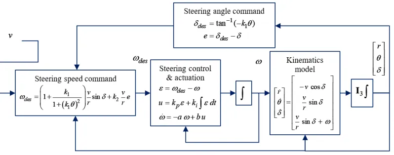
Figure 2. Overall smooth path planning (SPP) scheme depicts the smooth path planner (SPP) scheme at a glance, consisting of all the factors described above.

Figure 2. Overall smooth path planning (SPP) scheme

1, 2, p& i

k k k k are design parameters whose values are usually determined with the help of

simulation. k₁ determines how much reaction should be given to

θ

, and canranges from 0 to 10. k₂

determines how fast

δ

should approach

δ

_des and can ranges from 1 to 5. The choice of k_p&k_i

3

Experimental Results of Smooth Path Planner

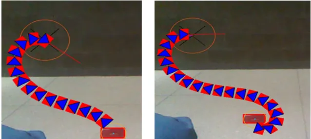
The SPP was applied to self-parking maneuvers of an experimental miniature mobile robot, as shown in Figure 3. An overhead camera looking downward was used measure the variables r,

θ

&

δ

. The steering command (5) & (11) was computed and sent to drive the robot to its predetermined target location & orientation.

Figure 3. SPP is applied to an actual miniature mobile robot. The triangular arrows emulate position and orientation of the robot.

4

Matlab Visualization of Smooth Path Planner

Once the SPP algorithm was established, it becomes a matter of formulting problems at hand to suit the algorithm, Figure 4 shows a Matlab animation of SPP used for single file, platooning maneuver. Here, the 2nd _{vehicle follows the lead vehicle. The 3}rd _{follows the 2}nd_{, etc.}

Figure 5 simulates the left turn maneuver at a junction, where the EgoVeh waits till the traffic clears before engaging the SPP scheme.

Figure 5. SPP for turning left at a traffic cross road.

The simplicity of the SPP calculation allows it to be used in more commplicated scenarios.

Figure 6 shows how the prime vehicle switches from LeadVeh1 to LeadVeh2, in the middle of a maneuver.

5

ROS Gazebo Simulation of Smooth Path Planner

A 3D simulation of leader-follower platooning for multiple Polaris Gem e2 vehicles was implemented using the Robotics Operating System (ROS) Gazebo simulator. Implementation in ROS is being investigated as we are preparing for real-time experimentation of the SPP schemes. Figure 7 shows four follower vehicles led by a lead vehicle swerving through a field, while Figure 8 shows a similar scenario that includes lane following maneuvers.

6

Discussions

Several aspects of this approach require further investigations and development. As noted in Section 2, practical measurements of the variables would need to be determined from a combination of measurements from camera, GPS, IMU, lidar and/or radar. Issues associated with noise, accuracy, multi-sampling rates need to be addressed.

A next aspect is to include the dynamics and control behaviors of the vehicle motion in the SPP analysis. This will take actuation drives, control schemes and processing delays into consideration so we can arrive at a more realistic expectation. We are presently in the process of realizing the SPP on Polaris Gem e2 class vehicles, with multi-sensors, for the 2019 IGVC. See Figure 8.

Figure 9. Gem e2 vehicles for testing the SPP

SequoiaSD GEM e2 Vehicle

Figure 7.Gazebo simulation of a lead vehicle and two followers performing lane keeping

maneuvers with the smooth path planner.

7

Conclusion

Even though the smooth path planner (SPP) was derived using detail analysis involving kinematics model, Lyapunov stability criterion and back-stepping control, its synthesis is relative simple. This allows the SPP to be readily adapted or switched to work with many car maneuvers. The formulation and simulation of the SPP in this paper show potentials for practical applications. This paper sets the foundation and validates ideas and scenarios for eventual actual realization of the schemes.

References

J. Park and B. Kuipers, May 2011, “A smooth control law for graceful motion of differential wheeled mobile robots in 2D environment,” 2011 IEEE International Conference on Robotics and Automation (ICRA), pp. 4896-4902.

W. Wadsworth & K. Chen, 1993, Linear Networks and Systems (book style), Belmont, CA. pp. 123– 135.

K. Iyengar, Aug. 2015, "Smooth control path planning and tracking of an autonomous mobile robot in real-time,”, M.Sc. Thesis, School of Engineering. and Computer Science., Oakland University, Rochester, Michigan, USA.

Olson, Edwin. 2004, "A primer on odometry and motor control."

C. S. Hargadine, 2017, “Mobile robot navigation and obstacle avoidance in unstructured outdoor environments,” Dissertation, Naval Postgraduate School, Monterey, California,

https://en.wikipedia.org/wiki/Lyapunov_stability

https://en.wikipedia.org/wiki/Backstepping

https://wiki.nps.edu/dashboard.action. Naval Postgraduate School, U.S. Navy, 2018,