16
Analysis of Vendor Managed Inventory System
Element Using ANOVA Method: A Case Study
Jitender
1, Sh. Vijay Kumar
2, Parteek
31
Research Scholar, Department of Mechanical Engineering, Sat Priya Group of Institutions, Rohtak, Haryana
2,3
Assistant Professor, Department of Mechanical Engineering, Sat Priya Group of Institutions, Rohtak, Haryana
ABSTRACT
In Vendor managed inventory a supplier of good ,usually the manufacturer, is responsible for optimizing the inventory held by a distributor.VMI requires a communication link-typically electronic data interchange or the internet –that provide the supplier with the distributor sales and inventory data it needs to plan inventory and place order. in contrast ,under the traditional arrangement the distributor handle those tasks The inventory can be owned by the distributor, or by the supplier . In this paper survey of 20 industries was carried out. On the basis of the mean calculated for different elements of VMI on 0-80 scale, all the elements were analyzed and plotted on a scatter chart, from where most important and less difficult elements were found out. Analysis of the data has done with the help of the XY Scatter Chart which is drawn between importance as abscissa and difficulty as . . After identifying the elements from XY scatter chart, apply the ANOVA analysis on those elements. From the result of the ANOVA analysis, we have checked the value is significant. This study help in finding VMI element which are most important and easy to implement
Key words: VMI, Inventory, Anova method, Forecast
INTRODUCTION
Vendor Managed Inventory simply means the vendor (the Manufacturer) manages the inventory of the distributor. The manufacturer receives electronic messages, usually via EDI, from the distributor. These messages tell the manufacturer various bits of information such as what the distributor has sold and what they have currently in inventory. The manufacturer reviews this information and decides when it is appropriate to generate a Purchase Order. The basic principle of VMI is that the vendor, or supplier, becomes responsible for managing the inventory at the customer’s site. In contrast to buyers who often manage a broad portfolio of purchased items, suppliers are usually responsible for a more limited range of products of which they have more specific knowledge, and therefore should be better in forecasting and managing the flow of their products through to the end consumer. Making the supplier responsible for replenishment should result in inventory and logistics costs being reduced throughout the total supply chain.
In order for the supplier to be able to manage this inventory, information about inventory levels, expected demand, promotional activities, and product related costs should be made available to the supplier by the buyer. This information enables the supplier to make better replenishment decisions based on total supply chain costs, and prevent local sub-optimization when both players would try to optimize their own profits individually. Early availability of such information enables the supplier to be pro-active, which should result in reduced lead times. Effective implementation of VMI thus requires a cross-functional and inters organizational approach. Accurate and timely demand information needs to be shared between the marketing and supply functions of the buyer as well as with the planning function of the supplier.
LITERATURE REVIEW
Lee et al. [1997] identified four major causes of the bullwhip effect – Demand forecast updating, the rationing gaming, order batching and price variations.
17 rather than introducing new problem specific systems solutions for new business requirements.
DALE D. ACHABAL [2000] describes the market forecasting and inventory management components of a Vendor Managed Inventory (VMI) decision support system and how this system was implemented by a major apparel manufacturer and over 30 of its retail partners.
N. C. Simpson [2001] model the order picking function and to explore the role of inventory stock levels in achieving economies of scale across this function in a deterministic demand environment.
S. M. Disney [2002] designed a VMI for various different ratios of production adaptation cost and inventory holding cost. A decision support system using causal loop diagrams and difference equations is proposed to determine the optimum design parameters in the vendor managed inventory, automatic pipeline, inventory and order based production control system (VMI-APIOBPCS) by relating it to the gain on demand when setting safety stocks at the distributor.
S. M. Disney [2003] modelled three different scenarios – a traditional supply chain, an internal consolidation scenario (with batching in the order rule) and the VMI supply chain to investigates the impact of a vendor managed inventory (VMI) strategy upon transportation operations in a supply chain.
Hansheng Suo [2004] said that Supply chain inefficiencies can result from incompatible incentives provided by independent decision-makers and also their risk aversion effect.
Haifeng, Guo Xiaoyuan [2005] studied The optimization policy of the purchase price and the profit under vendor managed inventory (VMI) and established a supply chain mode of VMI For a salable product, which is based on deterministic demand, having initial stock and having stock-out cost. In his analysis, VMI is found to increase profits of the buyer in the short-term motivation.
YU YUGANG [2006] discussed a VMI supply chain where a manufacturer and multiple retailers play a game with each other under partial co-operation in the inventory control with
Tinglong Zhang [2007] discussed an integrated vendor-managed inventory model based on the assumption that the buyer’s cycle times may be different and the vendor’s production cycle is an integer multiple of each buyer’s replenishment cycle
Peter B. Southard [2008] compared the costs of inventory systems used in practice by rural farm cooperatives to possible technology- enabled systems. Performance was measured in inventory costs, delivery costs and stock outs.
Yuliang Yao [2008] construct an analytical model to analyze the benefits realized for manufacturers and retailers under information sharing (IS), continuous replenishment programs (CRP) or vendor managed inventory (VMI) and compare the distribution of benefits between manufacturers and retailers.
W.K. Wong [2009] proposed a model in the context of a two-echelon supply chain with a single supplier serving multiple retailers in vendor-managed inventory (VMI) partnership. The proposed model demonstrates that the supplier gains more profit with competing retailers than without as competition among the retailers lowers the prices and thus stimulates demand.
G.P. Kiesm¨uller [2010] propose three different VMI strategies, aiming to reduce the order picking cost at the upstream location and the transportation costs resulting in reduced total supply chain costs. He compared VMI strategies are compared with a retailer managed inventory strategy for two different demand models suitable for slow moving products and found that if inventory holding costs are low, compared to handling and transportation costs, efficiencies at the warehouse are improved and total supply chain costs are reduced.
Jun-Yeon Lee [2011] presented and analyzed a simple periodic-review stochastic inventory model to examine the benefits of VMI from economies of scale in production/delivery in a global environment characterized by exchange rate uncertainty and large fixed costs of delivery.
18 decides how to manage the system-wide inventories of its fast deteriorating raw material and its slowly deteriorating product and accordingly develop an integrated model to calculate the total inventory and deterioration cost for such a system.
Model of ANOVA Technique:-
One way ANOVA: - Under the one way ANOVA, we consider only one factor and then observe that the reason for said factor to be important is that several possible types of samples can occur within that factor. We then determine if there are differences within that factor. The technique involves the following steps:-
(i) Obtain the mean of each sample i.e. obtain X 1, X 2, X 3, X 4 ………X k
Where there are k samples.
(ii) Work out the mean of the sample means as follows:
X = x + x1No .of samples (k) + x2 +⋯…………,x3 k
(iii) Take the deviations of the sample mean from the sample means and calculate the square of such deviations which may be multiplied by the number of items in the corresponding sample, and then obtain their total. This is known as the sum of squares for variance between the sample (or SS between). Symbolically, this can be written:
SS between = n1 X 1 − X 2 + n2 X 2 − X 2 + ……. + nk X k − X 2
(iv) Divide the result of (iii) step by the degree of freedom between the samples to obtain variance or mean square (MS) between samples. Symbolically, this can be written:
MS between =SS between N − 1
where (N-1) represents degree of freedom (d.f.) between samples.
(v) Obtain the deviations of the values of the sample items for all the samples from corresponding means of the samples and calculate the squares of such deviation and then obtain their total. This total is known as the sum of squares for variance and then obtains their total. This total is known as the sum of squares for variance within samples (or SS within), Symbolically this can be written as:
SS within = X1i− X 1 2 + X2i− X 2 2 +…….. + Xki− X k 2
i = 1, 2, 3…
(vi) Divide the result of (v) step by the degree of freedom within samples to obtain the variance or mean square (MS) within samples. Symbolically this can be written as:
MS within =SS within (n − k)
where (n-k) represents degree of freedom within samples. n= (total number of items in all the samples i.e. n1+n2+……. +nk ) - 1
k=number of samples-1.
(vii) For a check, the sum of squares of deviations for total variance can also be worked out by adding the squares of deviations when the deviations for the individual items in all the samples have been taken from the mean of the sample means. Symbolically, this can be written:
19 i = 1, 2, 3…
j = 1, 2, 3…
This total should be equal to the total of the result of the (iii) and (v) steps explained above i.e. SS for total variance= SS between + SS within
The degree of freedom for total variance will be equal to the number of items in all samples minus one i.e., (n-1). The degree of freedom for between and within must add up to degree of freedom for total variance i.e.
n − 1 = k − 1 + n − k
This fact explains the additive property of the ANOVA technique. (ix) Finally, F-ratio may be worked out as under:
F-ratio = MS betweenMS wit hin
This ratio is used to judge whether the difference among several means is significant or is just a matter of sampling fluctuation. For this purpose we look into the table, giving the value of F for given degree of freedom at different levels of significance. If the worked out value of F, as stated above, is less than the table value of F, the difference is taken as insignificant i.e. due to chance and the null hypothesis of no difference between sample means stands. In case the calculated value of F happens to be either equal or more than its table value, the difference is considered as significant (which means the samples could not have come from the same universe) and accordingly the conclusion may be drawn. The higher the calculated value of F is above the table value, the more definite and sure one can be about his conclusions.
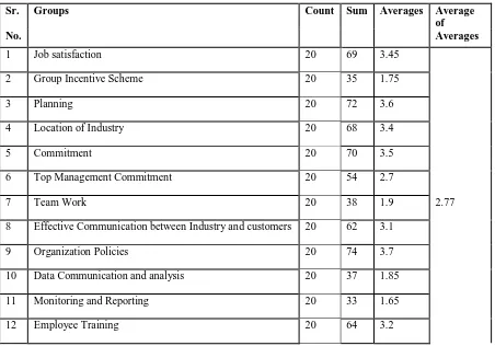
1.1.1. Result of ANOVA Analysis of Degree of Importance ANOVA: SINGLE FACTOR
Table 4.5: Averages of Elements for Anova
Sr. Groups Count Sum Averages Average
of
No. Averages
1 Job satisfaction 20 69 3.45
2 Group Incentive Scheme 20 35 1.75
3 Planning 20 72 3.6
4 Location of Industry 20 68 3.4
5 Commitment 20 70 3.5
6 Top Management Commitment 20 54 2.7
7 Team Work 20 38 1.9 2.77
8 Effective Communication between Industry and customers 20 62 3.1
9 Organization Policies 20 74 3.7
10 Data Communication and analysis 20 37 1.85
11 Monitoring and Reporting 20 33 1.65
20
13 Employee feedback and suggestion 20 63 3.15
14 Top Management Support 20 55 2.75
15 Customer feedback & suggestion 20 39 1.95
16 Frequent and Reliable Service 20 68 3.4
17 Customer Satisfaction 20 71 3.55
18 Customer Awareness 20 34 1.7
19 Multifunctional workers 20 30 1.5
20 Standardization 20 73 3.65
Table 1.1 indicates that Organization Policies has got the maximum value (i.e. 74), hence is the most important element of VMI for Industries and Standardization got 73, as mean score, which is second most important element of VMI whereas, Multifunctional has got 30 as mean, which is the least one, hence it can be termed as least important in manufacturing industry.
From Table 1.1, other most important elements are Planning ,Customer satisfaction ,Commitment, Job satisfaction ,Location of Industry, Frequent and reliable service, Employee training. Employee feedback and suggestion Table 1.1 also reveals the least important elements and these elements are Effective Communication between Industry and customers, Top Management Support, Top Management Commitment, Customer feedback & suggestion, Team Work, Data Communication and analysis, Group Incentive Scheme, Customer Awareness, Monitoring and Reporting, Multifunctional workers
Average of Averages =
3.45+1.75+3.6+3.4+3.5+2.7+1.9+3.1+3.7+1.85+1.65+3.2+3.15+2.75+1.95+3.4+3.55+1.7+1.5+3.65 20 = 2.77
SS between groups =
20[(3.45-2.77)2 + (1.75-2.77)2 + (3.6-2.77)2 + (3.4-2.77)2 + (3.5-2.77)2 + (2.7-2.77)2+ (1.9-2.77)2+ (3.1-2.77)2 + (3.7-2.77)2 + (1.85-2.77)2 + (1.65-2.77)2 + (3.2-2.77)2 + (3.15-2.77)2 + (2.75-2.77)2 + (1.95-2.77)2+ (3.4-2.77)2+ (3.55-2.77)2 + (1.7-2.77)2+ (1.5-2.77)2 + (3.65-2.77)2
= 249.95
MS between groups =249.95 N − 1 =
249.95 20 − 1=
249.95
19 = 13.16
SS within groups =
103.51+29.313+128.8+95.8+107.25+52.45+24.05+120.05+152.45+25.113+41.613+95.2+105.61+ 61.813+23.013+103.8+123.01+48.45+41.25+138.61
= 1621
MS within groups =1621 n − k=
1621 399 − 19=
1621 380 = 4.26
F − ratio =MS between MS within =
21 Table 4.6: Calculation of F-Ratio
Source of Variation SS d.f. MS F-ratio 10% F limit
Between Groups 249.45 19 13.16 3.08 1.45
Within Groups 1621 380 4.26
Total 1870.45 399
From the above table we can say that F- critical is less than the calculated F value. So we can say that the values of elements are significant.
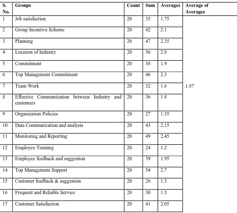
4.5.5 Result of ANOVA Analysis of Degree of Difficulties ANOVA: Single Factor
Table 4.5: Averages of Elements for ANOVA
S. Groups Count Sum Averages Average of
No. Averages
1 Job satisfaction 20 35 1.75
2 Group Incentive Scheme 20 42 2.1
3 Planning 20 47 2.35
4 Location of Industry 20 56 2.8
5 Commitment 20 38 1.9
6 Top Management Commitment 20 46 2.3
7 Team Work 20 32 1.6 1.87
8 Effective Communication between Industry and customers
20 36 1.8
9 Organization Policies 20 27 1.35
10 Data Communication and analysis 20 43 2.15
11 Monitoring and Reporting 20 49 2.45
12 Employee Training 20 24 1.2
13 Employee feedback and suggestion 20 39 1.95
14 Top Management Support 20 54 2.7
15 Customer feedback & suggestion 20 26 1.3
16 Frequent and Reliable Service 20 30 1.5
22
18 Customer Awareness 20 23 1.15
19 Multifunctional workers 20 25 1.25
20 Standardization 20 34 1.7
Table 1.2 indicates that Location of Industry has got the maximum value (i.e. 56), hence is the most difficult element of VMI for Top Management Support 54, as mean score, which is second most difficult element of VMI whereas, Customer Awareness has got 23 as mean, which is the least one, hence it can be termed as least difficult in manufacturing industry.
From Table 1.2, other most difficult elements are Effective Communication between Industry and customers , Job satisfaction , Standardization , Team Work , Frequent and Reliable Service, Organization Policies, Customer feedback & suggestion, Multifunctional workers, Employee Training, Customer Awareness
Average of Averages =
1.75+2.1+2.35+2.8+1.9+2.3+1.6+1.8+1.35+2.15+2.45+1.2+1.95+2.7+1.3+1.5+2.05+1.15+1.25+1.7 20 = 1.87
SS between groups =
20[(1.75-1.87)2 + (2.1-1.87)2 + (2.35-1.87)2 + (2.8-1.87)2 + (1.9-1.87)2 + (2.3-1.87)2+ (1.6-1.87)2+ (1.8-1.87)2 + (1.35-1.87)2 + (2.15-1.87)2 + (2.45-1.87)2 + (1.2-1.87)2 + (1.95-1.87)2 + (2.7-1.87)2 + (1.3-1.87)2+ (1.5-1.87)2+ (2.05-1.87)2 + (1.15-1.87)2+ (1.25-1.87)2 + (1.7-1.87)2 = 93.63
MS between groups =93.63 N − 1=
93.63 20 − 1=
93.63 19 = 4.93
SS within groups =
75.313+46.05+39.613+111.2+46.05+38.45+42.8+32.2+117.11+51.113+34.013+117.2+89.013+58.45+82.45+65.25 +77.013+102.61+87.813+30.45
= 1344
MS within groups =1344 n − k=
1344. 399 − 19=
1344
380 = 3.53
F − ratio =MS between MS within =
4.93 3.53= 1.51
Table 4.6: Calculation of F-Ratio
Source of Variation SS d.f. MS F-ratio 10% F limit
Between Groups 93.63 19 4.93 1.51 1.45
Within Groups 1344 380 3.53
23 Table 1.3 Elements Which Are Important As Well As Easy To Implement
VALUE OF VALUE OF
S.
ELEMENT MEAN FOR MEAN FOR
NO. IMPORTANCE DIFFICULTY
(0-40) (0-40)
1 Organization policy 74 27
2 Standardization 73 34
3 commitment 70 38
4 Job satisfaction 69 35
5 Frequent and reliable service 68 30
6 Employee training 64 24
7 Employee feedback and suggestion 63 39
8 Effective communication between
industry and customer 62 36
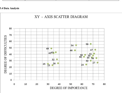
3.4 Data Analysis
Analysis of the data has done with the help of the XY Scatter Chart which is drawn between importance as abscissa and difficulty as ordinate. The axis crosses at their relative value of population mean (μ) i.e. for X axis it is 40 and for Y axis its value is 40. In figure , the lower right quarter i.e. Part-1 shows those elements of VMI which are Less important and are more difficult to implement. The upper right quarter i.e. Part-2 shows those elements which are highly important but are more difficult to implement. The upper left quarter i.e. Part-3 shows those elements which are most important and less difficult to implement in industry.
The lower left quarter i.e. Part-4 shows those elements which are less important but are easy to implement.
35 42 47 56 38 46 32 36 27 43 49 24 39 54 26 30 41 23 25 34 0 10 20 30 40 50 60 70 80
0 10 20 30 40 50 60 70 80
D
E
G
R
E
E
O
F
D
IF
F
IC
U
L
T
IE
S
DEGREE OF IMPORTANCE
24 REFERENCES
[1]. Dale D. Achabal, Shelby H. Mcintyre, Stephen A. Smith, Kirthi Kalyanam, “A Decision Support System for Vendor Managed Inventory”, Journal of Retailing, Volume 76, Number 4, 4th Quarter 2000,
[2]. Haifeng, Guo Xiaoyuan, “Optimization purchase price and the profit policy under vendor managed inventory”, Journal of Systems Engineering and Electronics, Issue: 2, Volume: 16.
[3]. Hansheng Suo, Jingchun Wang and Yihui Jin, “Coordinating a loss-averse newsvendor with vendor managed inventory”, IEEE International Conference on Systems, Man and Cybernetics, 2004.
[4]. Jan Holmstrom,” Business process innovation in the supply chain – a case study of implementing vendor managed inventory”, European Journal of Purchasing & Supply Management, Volume 4, Issues 2–3, June 1998,
[5]. Jun-Yeon Lee, Louie Ren, “Vendor-managed inventory in a global environment with exchange rate uncertainty”, International Journal of Production Economics, Volume 130, Issue 2, April 2011.
[6]. LEE, Hau L., PADMANABHAN, V and WHANG, Seungjin. The Bullwhip Effect in Supply Chains. Sloan Management Review (MIT: Maassachusetts Institute of Technology), Vol. 38, No. 3, 1997.
[7]. N. C. Simpson, S. Selcuk Erenguc, “Modeling the Order Picking Function in Supply Chain Systems: Formulation, Experimentation, and Insights”, IIE Transactions, 33(2),
[8]. Peter B. Southard, Scott R. Swenseth, “Evaluating vendor-managed inventory (VMI) in non-traditional environments using simulation”, International Journal of Production Economics, Volume 116, Issue 2, December 2008,
[9]. S.M. Disney, A.T. Potter, B.M. Gardner, Transportation Research Part E: Logistics and Transportation Review, Volume 39, Issue 5,September 2003,
[10]. S.M. Disney, D.R. Towill, “A procedure for the optimization of the dynamic response of a Vendor Managed Inventory system”,Computers & Industrial Engineering, Volume 43, Issues 1–2, 1 July 2002
[11]. Tinglong Zhang, Liang Liang, Yugang Yu, Yan Yu, “An integrated vendor-managed inventory model for a two-echelon system with order cost reduction”, International Journal of Production Economics, Volume 109, Issues 1– 2, September 2007 .
[12]. Yugang Yu, Zheng Wang, Liang Liang, “A vendor managed inventory supply chain with deteriorating raw materials and products”, International Journal of Production Economics, Volume 136, Issue 2, April 2012,
[13]. Yuliang Yao, Philip T. Evers, Martin E. Dresner, “Supply chain integration in vendor-managed inventory”, Decision Support Systems, Volume 43, Issue 2, March 2007