An Algorithm in the Process of Planning of Safety Pathway – a Collision-Free Pathway of a Robot

INTRODUCTION

The approaches to planning robot trajectories in an obstacle-based environment are based on optimisation methods. With a broad extent of the task, the optimisation methods require demand-ing calculations, which often make it impossible to solve the task in real time. The two problems complicate the solution of the real-time avoid-ance of collision:

1. The task is generally dynamic, because it is nec-essary to analyse the movement around an ob-stacle, taking into consideration the inaccuracy, uncertainty of the action of the robot, changes in the activities of the robot in time, etc.

2. Given the limited time of motion analysis, it is difficult to divide the stages of detecting ob -stacles and planning trajectories.

Industrial robot pathway planning

Planning motion in an obstacle environ-ment is a basic and current task. In order for

a robot to be able to plan its movement on its own, it needs to have the information about the state of the environment in which it is located and the criteria that have been set to determine the optimal route, the pathway. The information about the surrounding environment is obtained by the robot through the entries provided by the operator and automatically by sensors. An internal environment model (a map) is created from this information [1, 2]. The map is passed to an algorithm that calculates the destination pathway.

The resulting path connects the starting position with the target point, avoids obstacles and is optimal according to the specified crite-rion. The optimality criterion can involve e.g. finding the shortest path, the safest path, the fastest path (only through a familiar environ-ment) or a combination of these. One of the main goals of contemporary robotics research is to equip the robotic system with the basic capabilities it needs for intelligent and autono-mous behaviour.

An Algorithm in the Process of Planning of Safety Pathway –

A Collision-Free Pathway of a Robot

Naqib Daneshjo

_{, Cecilia Olexová}

_{, Marián Králik}

_{, Enayat Danishjoo}

1 _{Faculty of Business Economics with seat in Kosice, University of Economics in Bratislava, Slovakia}

2 _{Slovak University of Technology in Bratislava, Faculty of Mechanical Engineering, Namestie slobody 17, 81231} Bratislava, Slovakia

3 _{THK Rhythm Automotive GMBH, Duesseldorf, Germany}

* Corresponding author’s e-mail: [email protected]

ABSTRACT

The paper was based on research tasks in the field of robotics. It approaches solving the collision states of a

robot while operating equipment and applies the knowledge in the CATIA system environment. Motion Plan-ning is of paramount importance in robotics, where a goal is to determine a collision-free, unobstructed path for a robot that works in an environment which contains obstacles. An obstacle can be an object that is found in the robot’s workspace.

Keywords: collision states of a robot, motion planning, robot’s workspace, CATIA Volume 13, Issue 3, September 2019, pages 16–23

https://doi.org/10.12913/22998624/110154

Research Journal

Advances in Science and Technology Research Journal Vol. 13(3), 2019

A description of the robot environment – the analysis of selected solutions

The robot performs tasks in a constantly changing environment, to which it must constant-ly adapt to, leading to a continuous improvement of the robot’s perception and software. The en-vironment of this robot can be divided into two basic groups: a static environment (the robot’s environment and obstacles do not change), and a dynamic environment –that undergoes constant changes, and a robot or manipulator must con-stantly adapt to that environment. In our case, it is the static environment, so the environment is fixed. The robot environment was created in the CATIA system. In general, the robot’s workspace can have [5, 7, 9]:

1. The theoretical working space of the robot is the real space in which the robot is located, performs a work there and it is understood as a set of all points that are theoretically achiev-able by the end effector. A position in this space is given in Cartesian coordinates x, y, z. In the robot’s technical documentation, this space is referred to as the workspace.

2. The unusable workspace of the robot is the space in which is covered by different parts of the robot or the necessary peripheral devices and is therefore not achievable by the end effector.

3. The actual robot workspace is determined by the difference between the theoretical and un -usable robot workspace.

4. The safety area of the robot is located above

the workspace of the robot, which is the space that cannot be reached by the robot’s end-effec -tor, but the operator must not stay in that space during the robot’s operation.

The analysis of selected solutions

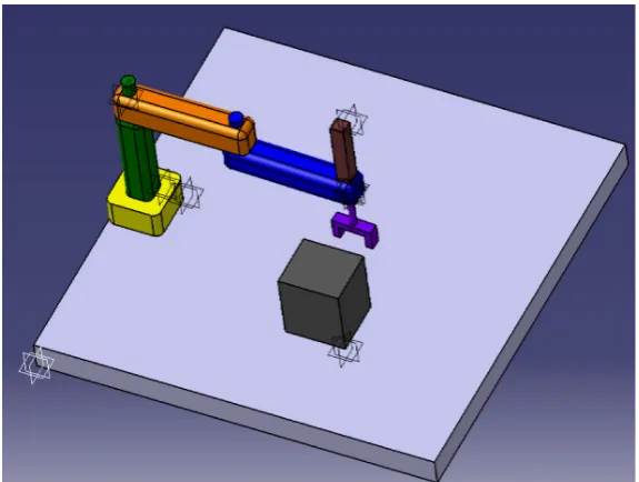
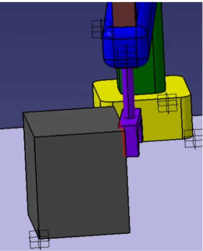
The robot’s environment is created by the ob-stacles that should be avoided in order to prevent collision. As an example, we create an obstacle for the robot in its workspace, by placing a bar-rier into the workspace. In our case, it will be a cube or a block that has defined dimensions and position relative to the location of the robot [3, 4]. We place the obstacle in the workspace so that a collision may occur. One obstacle is enough to approach the collision problem in the robot workspace, on the basis of which an example of the collision situation of the robot in the CATIA system and the subsequent creation of an algo-rithm for setting the collision-free pathway for the SCARA robot, also in the CATIA system will be demonstrated [6, 8].

The SCARA robot environment will be modelled and designed in the CAD/CAM CA-TIA environment. The advantage of this system is the simplicity and speed of designing a robot environment. Moreover, the simulation of this proposed system, will lead to a solution to this issue. This method of environment modelling is advantageous in off-line programming, where all parameters must be explicit in order to design, model and subsequently simulate individual mo-tions and possible collision states (Figure 1).

An important part of the robot analysis is the complete kinematic model of the mechanical sys-tem, which provides all the necessary kinematic quantities for the dynamic model of the mechani-cal system (force measure, cell loading, sizing), as well as for the needs of control (position and velocity regulator synthesis). It is about the prog-ress of the position and orientation of the end work point in time and the corresponding course of the position of the individual elements of the mechanism [6, 10, 11]. The location of articles is generally described in so-called generic coordi-nates (in robotics the term joint variables is often used) to indicate rotation, movement of individu-al motion axes.

The proposal of a solution algorithm design for the SCARA robot

The algorithmic approaches to robot motion planning are based on object-oriented, accurate, and discrete algorithmic techniques from which an effective solution is expected or anticipated. The algorithmic approaches to pathway planning emphasise the exact mathematical view of the problem with an exclusion of heuristics. It ex-amines the computational complexity and solv-ability using algorithms. For complex moving systems, these may not be feasible. For practical applications, heuristic scheduling approaches are probably necessary, which can be used to make the algorithm solutions more effective. The com -mon principle of algorithmic and heuristic solu-tions is the configuration space method. The basis of this method is the generalisation of the point pathway planning problem in the area of trans-formed obstacles.

A simple pathway from start to finish, usu -ally a straight line constitutes a hypothesis that is being tested for potential collisions. When col-lisions occur on the robot’s path, a new path is generated which bypasses the obstacles already found. When there are no obstacles in the robot’s pathway, an optimum pathway is designed to avoid any collision. The algorithm is required: 1. To find a safe path that involves moving around

obstacles.

2. To guarantee that these moves are as short as possible.

This algorithm can be divided roughly into 3 steps:

1. Calculating the volume of the changes of the moving object along the proposed pathway. 2. Determining the coverage of obstacles between

the robot’s pathway. 3. Suggesting a new pathway.

The algorithm for determining the kinematic parameters can be summarised as follows:

• Draw a simplified robot scheme.

• Number each robot joint from 0 to n, with 0 – th being the robot coordinate system.

• The coordinate system variables in the joints between (i-1) and i denote by the index i.

• Orient the vector z for the i- th joint with the axis of rotation at the pivot joint, or with the translation axis for the sliding connection.

• Determine numerical values ai as minimum distances between z_i-1 a z_i and z_i,

• Determine numerical values d_i as minimum distances between x_i-1 and x_i.

• Determine q_i, angle of rotation, in the positive direction in the clockwise coordinate system around the axis z_i-1, i.e. between the axes x_i-1 and x_i.

• Determine α_i, angle of rotation, in the posi-tive direction in the clockwise coordinate sys-tem around the axis x_i, i.e. between the axis z_i-1 and z_i.

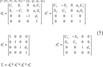
The position and orientation of the i-th co-ordinate system of the respective kinematic chain link of the robot can be transformed into (i-1) coordinate system by means of a matrix as a product of four homogeneous transformation matrices, denoted as Denavit–Hartenberg matrix, referred to as D–H matrix in world literature, or the A-matrix.

A_i-1,i = Rot(z, q_i )*Trans(0,0, d_i)* Trans(a_i,0,0)* Rot(x, α_i) (1) and after substituting the appropriate parameters into the transformation matrices we obtain the resulting Denavit–Hartenberg transformation matrix:               1 0 0 0 cos sin 0 sin * sin * cos cos * cos sin cos * sin * sin cos * sin cos i i i i i i i i i i i i i i i i i d a a              

Ai-1,i =

(2)

If you choose the n – th coordinate system of the robot effector, multiply A – matrices:

Advances in Science and Technology Research Journal Vol. 13(3), 2019

We obtain a known matrix that contains the position and orientation of the robot’s effector relative to the robot coordinate system, i.e.

   

 

   

 

1 0 0

0z z z z

y y y y

x x x x

p a o n

p a o n

p a o n

Te = ₍₄₎

The above-mentioned mathematical appara-tus is also the basis for the detailed design of the handling operation as well as for testing a colli-sion of a robot with the operated equipment dur-ing the implementation of the assembly process itself. The robot with its kinematic chain should avoid a device – an obstacle in its working space. For a given position and orientation of the robot’s effector, which is given e.g. by the conditions of the assembly operation, it is necessary to calcu-late the angles of rotation and movement in the individual kinematic pairs (joints) of the robot. We are talking about the so-called inverse role of the kinematics. It is a relatively complicated task, which is still at the forefront of many workplaces in the world. Inverse transformation algorithms are becoming faster and more versatile. The ba-sic criterion for inverse transformation methods is their versatility, i.e. using the same algorithm for any kinematic structure and the number of degrees of freedom of the robot. Universal meth-ods are applied mainly to the large CAD systems when the programming system has to handle an inverse kinematic role of any kinematic structure. For the management application, the speed of the calculation is decisive, because the inverse task solution ideally takes place in real time [4, 7].

The kinematic structure of the SCARA-type robot (Fig. 2) is composed of an arm mounted on a central column by a swivel joint and coupled to another arm (forearm) also by a joint. At the end of this second arm, there is a vertical sliding joint, in which the slide arm moves to provide move-ment of the robot’s effector in the z-axis. Accord -ing to the principles of Denavit and Hartenberg, coordinate systems can be assigned to individual joints and four transformation matrices can be assembled [11, 12]. The first expresses the trans -formation of the first arm to the basic coordinate system and the other matrices express the trans-formation relationship according to the Denavit– Hartenberg convention.

q= [θ1, θ2, d3, θ4] = [q1, q2, q3, q4]

(5)

In order to express the overall transformation along the kinematic chain of the robot, we obtain the resulting transformation matrix:

(6)

In order to simplify the recording, substitu-tions were used for trigonometric funcsubstitu-tions:

S₁ = sinθ_1, C₁ = cosθ₁.

Similarly, for other angles, abbreviated notes: S2, C2, S4, C4 were used. The notation was used for the sums of the trigonometric functions:

S_1–2 = sin(θ₁+θ₂), C_1–2 = cos(θ₁+θ₂)

In order to calculate the inverse solution, it is necessary to obtain the individual articulated variables of the robot at the specified position of the end effector orientation. Therefore, we used the following formulas to calculate the sum and difference of the two angles of trigonometric functions:

sin (α ± β)= sin α cos β ± cos α sin β (7)

cos (α ± β)= cos α cos β ± sin α sin β (8) On the basis of the resulting matrix pertaining to the position and orientation of the robot effec -tor Te, the following formulae apply to determine the position:

px =

a

.

C



a

.

C

py=

a

.

S



a

.

S

pz = d₁q₃d₄

(9)

In the considered case, it was necessary to ex-press the joint variables θ₁, θ₂, θ₄, and d₃. We de-termined the value of the required arm extension from the specified position p_z and the values d_1, d_2, and d₄ that are given by the robot design

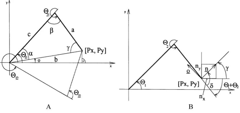
d₃ = p_z – d₁ – d₄. (10) However, for θ₁and θ₂, the two trigonomet-ric equations of two unknowns needed to be re-solved. In order to simplify the expression of these angles, the arms were translated into the horizontal xy plane. The shoulder positions al-ways form a triangle (Fig. 3). If the joint of the first arm is connected with the end of the other, where the position of the end effector in the xy plane is also present, the cosine sentence that ap-plies to the general triangle is:

a2 _{= b}2 _{+ c}2 _{– 2bc cos α (11)}

And then the following applies:

α = arccos((b2 _{+ c}2 _{– a}2_{)/2bc) (12)}

If the relevant parameters are substituted, for the calculation of the angle α, according to Fig-ure 1, the desired angles θ₁, θ₂ can be calculated. However, from Figure 3A, it can be seen that the task has two solutions. The first solution is denot -ed with the complementary index 1 (θ₁₂, θ₂₂) and

Table 1. Data to make d-h matrix for SCARA robot

os θ d a α

1 q1 d1 a1 π

2 q2 0 a2 0

3 0 q3 0 0

4 q4 d4 0 0

Figure 3. View of the robot arm horizontally:

A) The scheme determining angles θ₁ and θ₂; B) The scheme

Advances in Science and Technology Research Journal Vol. 13(3), 2019

the second with index 2 (θ₁₂, θ₂₂). The permissible solution also depends on the boundary conditions of the input, e.g. whether there is an obstacle in the robot’s space, a direction of the movement is required according to the designed manipulat-ing operation, the design limitations of the robot, etc. Finally, the angle of rotation of the last fourth joint should be expressed. The schematic repre-sentation can also be performed in the xy plane. Figure 3B shows the rotation of the joint relative to the previous robot cell. The joint always rotates around the z-axis, so the values of n_x, n_y, or the n_x, n_y. Since n and o are the unit vectors assigned to the robot gripper and their projections to the ro-bot’s basic coordinate system axes (x₀, y₀, z₀) are its directional cosines, then the rotation angle in this system can be directly determined:

γ = arctg(n_x / n_y) (13)

The angle of rotation of the second arm, rel-ative to the base coordinate system, can be ex-pressed as:

δ = θ₁ + θ₂ (14)

Then, for the sought angle θ₄, it holds:

θ₄ = γ + δ (15)

The collision-free pathway solution for the SCARA robot in CATIA system

After designing the environment for the SCARA robot and designing its construction it-self, it was necessary to define the position of the robot and the position of the obstacle. After

defining these positions, the joints and move -ments in each of the joints had to be determined. After defining these parameters, simulating, or solving collisions in the workplace with the ro-bot can be carried out. Thus, while designing a collision-free pathway, bypassing the obstacle, the following procedure was implemented:

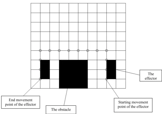
As shown in Figure 1, it is obvious that there are a lot of ways to implement a collision-free pathway. Therefore, it was necessary to limit the number of movement possibilities and propose individual paths for this limitation. The limita-tion involves the movement in individual joints by .rotating the first joint θ₁ and shifting in the third joint according to the scheme of Figure 2; the effector is left in the basic position as per the Figure 4. At the same time, it is the first variant of the collision-free pathway solution. The second option is to proceed in the same way, but rotate the effector by 90 degrees, see Figure 5.

In order to implement the pathway, it was nec-essary to determine the exact path from the start-ing point, denote it by the letter A and denote it by the letter B in the endpoint. As it can be seen from Figure 4 and 5, the configuration space, which is important for us, was converted from 3D envi-ronment to the 2D envienvi-ronment and divided into 10x10 configuration units. It was subsequently employed to facilitate designing any pathway and implement this collision-free pathway using the CATIA system.

In implementing of these two variations, as mentioned at the beginning, there are three op-tions for avoiding collisions while mobbing from the starting position (A) to the end position

(B). These three options can be summarized as follows:

1. In the first method i.e. the collision simulation; the effector collides with the obstacle as per the Figure 6, subsequently, one step back is taken and this position is used for pathway creation. Essen-tially, in this way of collision-free pathway for-mation, the surface of this obstacle is described. This method does not guarantee the shortest path, which is disadvantageous because the robot per-forms unnecessary movements. In real life, this method is not permissible because it increases production, handling time, etc., which is finan -cially ineffective, and of course, it increases the costs and the effort is to achieve the reduced costs.

2. The second method is built on the position of obstacles and positions of the robot. The ad-vantage of CATIA is that it is easy to measure the position and shoulders between the obsta-cle. Then, by creating the points (see Figure 4 in the second case 5) the collision-free path-way will be created, for the robot effector. A collision-free pathway is subsequently created for the avoidance of obstruction.

3. The third way is the visual simulation of the pathway. This pathway creation option is the easiest and time-saving. Visually then, in real time, suitable parameters of this pathway are set up, basically bypassing the obstacle to avoid collision, which should not happen, because all the rotations are made in real time, i.e. at the same time it visually controls the course of this pathway. This method is suitable for illustra-tion. Therefore, this method to was employed demonstrate this issue.

After implementing these three pathway cre-ation options, each simulcre-ation of these paths can be saved. The CATIA system allows transforming this model of environment with a robot and an obstacle and their simulation of the collision-free pathway into a robot programming system. This environment modelling system is beneficial in off-line robot programming.

CONCLUSIONS

With automatic motion planning and appro-priate sensors, a robot quickly adapts to unexpect-ed changes in the environment when modelling workspace errors. The basic function of intelli-gent robotic systems is the ability to perform a

Figure 5. Positioning of the effector after the turning by 90°

Advances in Science and Technology Research Journal Vol. 13(3), 2019

large number of tasks independently without ad-ditional information and to adapt to the continu-ous changes in the work environment.

The principle of solving of the problem is based on the kinematic analysis of the structure of the robot and the solution of the inverse trans-formation of the position and orientation of the robot’s effector to determine its position as an end part. The challenge was in line with the as-signment of the Master’s thesis on a robot with SCARA kinematics. Due to the level of difficulty in solving the challenge, appropriate tools were sought in order solve this problem. The CATIA system with the DMU kinematics module was used. In this environment, both the environment model and the robot itself were created. Then, two problems were solved by simulation meth-ods, namely the collision problem and the plan-ning of the collision-free pathway for the SCARA robot. The solution can be visually verified and is also convenient. This paper provides a closer in-troduction to the issue of collision in a workplace with a robot, in our case the SCARA robot.

A main benefit of the paper involves a design of the verified collision-free pathway of robot’s effector, thus shortening the program tuning pro -cess and avoiding the material damage caused by robot’s collision with the operated equipment.

Acknowledgement

This work has been supported by the Scien-tific Grant Agency of the Ministry of Education of the Slovak Republic (VEGA 1/0251/17)

REFERENCES

1. Berg, D.M., Otfreid, C., Kreveld, M., Overmars, M.: Computational geometry – Algorithms and ap-plications, Springer, 2008.

2. Angeles, J.: Fundamentals of robotic mechanical systems: Theory, methods, and algorithms, Second Edition. Springer, 2014.

3. Carbone, G., Gomez-Bravo, F.: Motion and Opera-tion Planning of Robotic Systems. Background and Practical Approaches. Springer, 2015.

4. Daneshjo, N., Majernik, M., Dudaš Pajerská, E. Danishjoo, M.: Methodological Aspects of Mod-elling and Simulation of Robotized Workstations. TEM Journal, 2 (2018). 293–300,

5. Daneshjo, N., Hajduova, Z., Dudas Pajerska, E., Danishjoo, E.: Design of dedicated automated de-vices with cad support. Modern Machinery Sci-ence Journal, March (2018), 2795–2799.

6. Daneshjo, N., Hajduová, Z., Dudaš Pajerská, E.,

Danishjoo, E.: Specification of the application of

vibrodiagnostics in assessing the state of the in-dustrial robot. Advances in Science and Technol-ogy – Research Journal. 13 (2019), 68–78.

7. Komak, M., Králik, M., Jerz, V.: The generation

of robot effector trajectory avoiding. Modern Ma -chinery Science Journal, June (2018), 2367–2372. 8. Fabian, M., Boslai, R., Ižol, P., Janeková, J., Fa

-bianová, J., Fedorko, G., Božek, P.: Use of para -metric 3D modelling – Tying parameter values to spreadsheets at designing molds for plastic injec-tion. Manufacturing Technology, 15 (2015), 24–31. 9. Manová, E., Čulková, K., Lukáč, J., Simonidesová,

J., Kudlová, J.: Position of the chosen industrial companies in connection to the mining. Acta Mon-tanistica Slovaca. Košice: Technical University of Košice, 23 (2018), 132–140.

10. Palko, A., Smrček, J.: The use of pneumatic artifi -cial muscles in robot construction. Industrial Ro-bot – An international journal. 1 (2011), 11–19. 11. Smrček, J. Palko, A., Tuleja, P.: Biomechanical

gripper – new mechanism effector for robots. Bu -dowa i eksploatacja maszyn. 12 (2004), 227–238. 12. Yatsenko, V.: Fast exact method for solving the