IJEEE, Vol. 3, Issue 5 (October, 2016) e-ISSN: 1694-2310 | p-ISSN: 1694-2426
REVIEW ON POINT SPREAD FUNCTION
ESTIMATION TECHNIQUES
1
Ritesh Pawar,
2Dr. Maitreyee Dutta
1,2Department of Electronics & Communication Engineering
National Institute of Technical Teacher Training & Research, Chandigarh (UT), India 1
Abstract- Real image is converted into blurred image by many factors. These factors are in the form of the defocus, motion blur, and gaussian blur and by capturing the image from the camera. These blurs are based on the function called as Point Spread Function. PSF is generally unknown for the blind image deconvolution. So for estimation of this function different techniques have different methods. In this paper different author has been taken different techniques for the restoration of the image. These techniques are based on the different parameters like standard deviation, PSNR for gaussian blur and motion blur and radius for defocus blur. The comparative analysis shows that in gaussian blur wiener filtering gives better results, for motion blur radon transformation and defocus blur two phase method gives better results for image restoration.
Index Terms: Defocus, Gaussian Blur, Motion Blur,
PSF.
I. INTRODUCTION
The estimation of the blind deconvolution and the blur kernel is very challenging and famous problem in the image processing and real world of computer vision [1]. In the many decades of image processing topic can produce several effects by standard linear inverse problem. So in real applications like remote sensing, photography, medical imaging, fluorescence microscopy, the point spread function cannot be determined more easily [2]. The PSF estimation can be determined with the help of the several techniques like patch based degradation, gradient domain correlation, edge prediction etc. Our main purpose to achieve the goal of estimating the true image F by the observed image G by the relation,
= ∗ + (1)
Here H defines as the PSF, N denotes the sample sets of the zero mean gaussian noise of variance σ2 and * represents the two dimensional convolution [3]. We can introduce the blur of an image with the help of the different camera stages. Also we can find the generally used sources of the image blur is motion, defocus, pixel size, sensor resolution, anti- aliasing filters on the sensor which can be produced by the aspects of the camera. Age can be deblurring using the deconvolution method, by the proper knowledge of the blur kernel. During the PSF estimation
the loss of the information during blurring has a common problem in a single blurred image. The partial constraints are found from the observed blur image from the solution. PSF estimation is used the different convolution techniques to match the desired image with different combination of the PSFs and sharp images [4]. Image degradation model is expressed in equation (2). True image is represented as F(x, y) in given equation, this image is able to seen as blurred image by the help of the image degradation system which is represented in the degradation system as function of H(x, y) and this function is also called as PSF of the degradation system. The true image or blurred image F(x, y) and the point spread function H(x, y) are convolved with each other by convolution function and the effective outcome is further influenced with noise signal N(x, y), after the convolution original image and blurred function over the influence of the noise the degradation system gives the output as degraded image in the form of G(x, y). An image is given by this function called as blurred image. This procedure is formulated as [5].
G (x,y) = H(x,y) * F(x,y) + N(x,y) (2)
In image processing deconvolution of the image is most important topic for several decades. Image processing has many real applications in which point spread function (PSF) can not be obtained more accurately and easily. So the process of the blind and non blind deconvolution occurs in the process. In the blind deconvolution the process of the estimation of the original image and the point spread function occurs simultaneously. But in the case of the non blind deconvolution first of all estimate the point spread function and then process the estimated image with non blind deconvolution to restored the original image [6].
function and given parameters the blur function can be assumed which give the results whoes does not match with the real imaging model of the optical devices which reduce the restoration execution. So to overcome this problem blind image super resolution process comes in effect, estimating the high resolution image and blur function at the same time. The main problem arises in the blind de-blurring is that it gives the incomplete convolution result. Cut off frequency destroyed the relationship between the convolution and boundaries and make the process more complicated to recognize the blur function of the image [8].
With the known PSFs the image deblurring is the method of improving the sharpen version of the blured image. Blurring process is generally the process of the convolution of the partial spread function with the original image and the process of the deblurring the image is called the inverse of the convolution which is known as deconvolution. Direct inverse filtering is the simplest method of the image deconvolution in frequency domain. From the inverse filtering the frequency response of the vagued image is calculated by spliting the image element wise by that of the partial spread function [9].
This paper is catagorized in four sections. In section 2 we discuss the estimation of blur parameters. Section 3 describes the PSF estimation techniques. Section 4 presents the simulation results. After estimating the blur parameters image restoration is done in section 5. In final section 6 , discussion of conclusion.
II. ESTIMATION OF BLUR PARAMETERS In the present section we are dicussing the blur parameters of image with the help of the gaussian noise, motion blur and Defocus step by step.
A. GAUSSIAN NOISE PARAMETER
When the process of the image restoration is done, then image can be ruined by the different types of noise. The most common noise are found is the gaussian noise. Gaussian noise parameter can be estimated by the different methods in image restoration process. The most common gaussian noise model is defined as:
n(a,b) =
πσ e
( ⁄ σ) (3)
From the above equation σ is standard deviation in gaussian noise model which is unknown in PSF estimation and some time it is to be assumed [10], [17] while estimating the PSF, the gaussian point spread function in different imaging systems is commonly used so to determine its parameters wiener filter is used. To identify these parameters e.g. point spread function size is estimated by setting the threshold value. The Gaussian PSF is generally used as the blur function in different optical measurements and imaging models. This function is generally described as:
G(m,n) = √ πδexp − δ (m + n ) , (m, n) ∈ R
0 Otherwise
(4)
Here standard deviationis defined by δ, supporting region
defined by the R, this R is used as the matrix size of L x L,
where L is odd number. So in this function basically two parameters are to be estimated, that are the standard
deviation (δ) and PSF size (L) with the help of the wiener filtering [11]. For the inverse gaussian group the two gaussian parameters are found with PDF. The homogeneity
of the scale like parameters λ is the main assumption for the inverse gaussian mean; these can be calculated by the given formula [12], [13], [15].
hx(x|μ,λ) = λ π
⁄
exp − λ
μ (x −μ)
(5)
Where x > 0 and λ > 0.The generalized gaussian distribution with probability distribution function is used in many cases like digital image processing, blind signal separation of speech etc. The GGD is a generalized form of the Gamma distribution family. GGD function with mean
μ, scale parameterβ and shape parameter α is defined as:
f(x:α,β,μ) = α βΓ( ⁄ )α
μ β
α
(6)
Where β = σ Γ( ⁄ )α Γ( ⁄ )α = σ
Γ( ⁄ )α
Γ( ⁄ )α ,Γ(z) =∫ e t dt ∞
is the
gamma function; -∞ < < ∞, > 0, > 0; and σ is
standard deviation [14]. In the parametric PSF estimation the blur stein’s unbiased risk estimation is depends upon the parameters of the gaussian (s, λ),these parameters can be estimated by minimization of the blur SURE with the help of the exact wiener filtering. The parametric PSF estimation can be characterized by the gaussian kernel as:
Gs(i , j ; s) = M∙ exp − (7)
Where s2 is the variance and (I, j) shows the 2D coordinates, M is the coefficient of the normalization. The projection operator PG is formulated for 1D in gaussian Blur parameter estimation is as [2], [16], [18]:
PG(f)(x) = m0Gs(x) =
√ π e (8)
B. MOTION BLUR PARAMETERS
In image restoration process degradation model can described in the form of uniform linear motion. Generally uniform linear motion has been taken because of the reason that sometime this motion taken as the non uniform linear motion in certain condition. The basic formula of the motion blur model in 2D plan is define below,
G (x,y) =∫ − ( ), − ( ) (9)
When relative motion occurs between the camera and object while capturing the image then motion blur is define in the form of a translational, a rotation and change in scale or combination of these. Uniform linear motion blur model generally defined in image restoration can be formulated as below in equation (10). Where parameter l defined as the
model is determined then the point spread function H(x,y) is also determined [19], [20].
H(x,y) = , + = 0, + ≤
0, ℎ (10)
When we calculate the Motion blur parameters over the directional and orientation pyramids then we can introduced the adaptive thresholding to compute the sharpened sub-bands of the edges of the image. This will help in reducing the sub-band value in to some small finite value [21]. The motion Blur is also modeled as in linear shift invariant and the formula is derived as
λ∫ − ( ) = λ∫ ⊛ ( ) ( )
= λ ⊛∫ ( ) ( )
= λ (y⊛hT)(x) (11)
The parameter hTbelongs to the motion blur PSF, while
δs(t) define as Dirac delta function at s(t) ∈ R 2
[22]. Frequency domain estimation is also used for motion blur image restoration process. This process is characterized by the PSF estimation which decomposed in to motion kernel and defocusing kernel. Further this motion kernel is estimated by the frequency domain, which performs the matching of the parameters in orientation and two axis lengths [23]. Motion blur angle detection most common Gabor filter is used, because when on applying the threshold value the small errors can cause the large variation in estimation of blur angle. The orientation parameters of filter give blur angle.
ℎ( , ) =
( ) ( )
(12)
( , ) = e − + × [− ( +
(13)
The function σxand σydenotes as standard deviation,ϕand
ω are the orientation and frequency of the Gabor filter [24]. Different types of motion blur may be distinguished between the relative motion of capturing device and picture. When picture is recorded with camera at a constant velocity and angle in horizontal axis on the exposure interval, then this may defined in 1D by defining the length of motion L= vrelativetexposure, then PSF is derived as [25]
B(x,y;L,ϕ)=
+ ≤ = −
0 ℎ (14)
Motion Blurred image in frequency spectrum shows the parallel lines gives very low values near to zero by orthogonal to motion orientation. For finding these dominant parallel lines we can choose different method like Radon transform, haugh transform, cepstral method or any other methods, these are discussed as below.
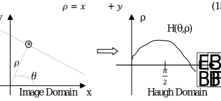
1. Haugh Transform Method
The haugh transform is used for patterns like lines, circles and ellipses in an image. This method is generally useful in line detection, which is depends on the polar representation of line
= + (15)
y ρ
H(θ,ρ)
π θ
Image Domain x Haugh DomainFig. 1 Haugh Transform
2. Radon Transform Method
Along the straight line the radon transform consist of integral function of the integral transform. These real valued functionϕ(x,y)∈R2, at angle θ and distance ρfrom
the origin is given in equation (16). Where δ denotes the
Dirac delta function. The modified radon transform define over two ways: (i) Radon transform with same area for different angle; (II) polar coordinate integration is formulated directly.
R( , , ) =
∫ ∫ ( , ) ( − − ) (16)
Y ρ R(θ,ρ)
θ
ρ π
x
Image Domain Radon Domain
3. Cepstral Method
Motion blur length estimation can found with the help of the radon transform and cepstral method. The cepstral transform can use for blur component and image components separation. It is defined in an image f(x,y) as follows [26],[10],[27],[28].
{ ( , )} = ( | ( ( , ))|)
(17)
C.
DEFOCUS BLUR PARAMETERSWhile taking a photograph some common type of blur is to be detected in the picture. These blur are in the form of the small number of pixels in the image that are comes in the frame due to defocus of the image. These small blurs contains the important clues of the depth of image. This type of blur is called as Just Noticeable Blur. These small blurs cannot distinguish with unblurred structure which is based on the local information. So to find this sparse edge representation and blur strength estimation is used.
min ‖y − Dx ‖ s.t.‖x ‖ ≤ k (18)
calculating the sparse edge we can find the blur strength estimation with the help of the formula given below, where a, b, c,d are fitted variables, σ is the standard deviationand f is the sparsity feature [29].
f = ( σ )+ d (19)
Spatially varying degradation model is also used for obtaining the defocus blur kernels, space invariant gaussian kernels can approximated region wise for defocus blur kernels and it may be restored in the form of FIR filter. Where G(x,y) is out of focus image and F(x,y) is in focused image, h(s,t) is space invariant PSF [30].
G(x, y) = ∑ ∑ h(s, t)F(x − s, y − t) +η(x, y) (20)
In single image estimation of spatially varying defocus blur is estimated by re blurred the image with the help of the gaussian kernel and defocus blur is estimated from ratio of the gradient of input and re blurred image.
∇i (x) = ∇ i(x)⊛G(x,σ )
= ∇((au(x) + b)⊛G(x,σ)⊛G(x,σ )
π σ σ
=exp −
σ σ (21)
Where standard deviation is defines for the re-blur gaussian kernel. Ratios of gradient magnitude between original and re-blurred edges are given in equation (22). The unknown blur amount is calculated by equation (23), [31], [33].
|∇ ( )|
|∇ ( )|= − − (22)
=|∇ ( )||∇ ( )| = , = (23)
In an image 2D map of scale parameter called defocus blur map in which different levels of local blur at each pixel is indicated. The PSF estimation scale for each pixel is depends upon the local probability estimation and coherent map estimation.
= ∑ ∑ ∇[ ]( ) , (24)
Where = 1 +
( )
(25)
Here ( ) is defined as defocus blur spectra and is optimal maximization of defocus blur. The coherent map estimation is achieved by minimizing the energy function, which consist of the data term and smoothness parameters. This parameter can control the strength of the constraints. R= {rx}xis defined as the whole pixel solution in image [32].
( ) = ∑ ( ) + ∑( , )∈ , ( , ) (26)
III. PSF ESTIMATION TECHNIQUE Image restoration process may achieve with the different types of the estimation techniques. Point spread function is estimated by various techniques in the blind image deconvolution.
A. Novel SURE Parametric PSF Estimation
In this paper author used a novel technique which is based on the blur SURE criteria used for the estimation of the PSF. This is a filtered version for MSE in blur estimation. Here the point spread function is the unknown parameter which is to be estimated. To estimate this unknown parameter from minimization they used wiener filtering. From this blur kernel estimation image deconvolution is done with the help of the proposed algorithm. This research shows that minimization of the blur SURE gives exact PSF estimation similar to exact point spread function when they use developed SURE based deconvolution algorithm [34].
B. Blind Image Restoration for PSF Estimation
In this paper for imaging model blur function is estimated with blind image restoration technique is used for enhancement in image for better quality. Here authors calculate parameters of the gaussian PSF of the image. Multiple curves of error are generated in different parameters by wiener filter algorithm. Size and standard deviation of PSF are estimated from these curves. Wiener filter is used for the restoration of the blurred image. From the experiment they shows that PSNR gets highest value around PSF and gets lowest when it is far away from point spread function [35].
C. Multiscale Patch Based Image Restoration
In this paper processing is based on the overlapping of the patches into the target image, restore the each patch separately and then by plain averaging merge the results for the final output. The prior techniques are focused on the intermediate results of patch, instead of the final outcomes from the restoration. So to overcome this problem expected patch log likelihood method was come in frame. In this paper author wants to extend that research and improve the EPLL by multi scale patches from the target image which are of the same size and the footprints of the target image changes due to sub sampling of the image. In the prior research of patch based restoration algorithm serves the local patch as global stochastic phenomenon. In this research the use of the multi scales EPLL by motivating the use of the simple gaussian case. This method is used for the image denoising, deblurring and super resolution [36].
D. Image Restoration by Wavelet Image Fusion
In this research authors want to show the new technique for the restoration of the image by fusion process. Firstly motion blurred image is recovered with LR and wiener filtering method. The new technique is applied then as for image fusion depends on wavelet process. From the research authors found this technique has good performance for image restoration [37].
E. Sparse and Adaptive Method
This technique is further used for the training dictionaries for the purpose of the showing image contents accurately. Here adaptive dictionary and sparse method used together for deblurring the image more accurately [38].
F. Radon Transformation and Bilateral Filter
For motion blur photography is the challenging task. Image is blurred due to long exposer time taken by camera. Camera high gain may cause the dark and noisy image with short exposer time. The proposed algorithm is used to remove these types of the effects. For this firstly check that from which factor image is blurred and then restore it from deconvolution process. In this paper blur kernels is estimated by blurred edges. These kernels are estimated by inverse Radon transform. The comparison is done in between wiener filter, LR, inverse filter and proposed method [39].
G. Sparse Representation for Blind Image Restoration
This research shows basic two dimensional patterns is modeled from blur kernel in the form of sparse linear combination. This technique is based on modeled method over competitive edge blur kernels, due to reason that this design is more flexible for dictionary design customization. This may help for various applications in the formation of adaptive design. Here Kronecker is used as a product for gaussian kernels. Authors also take the results in PSNR value and compare it with previous technique [40].
H. Mixed Gaussian and Impulse Noise Removal by Alternating Direction Method
In this paper Blurred image corrupted by gaussian noise and impulse noise together is restore with high order total variation method. This method is done with the help of the alternating direction method of multipliers. The demonstration of the results shows the efficiency of the proposed technique with its performance [41].
I. Two Phase Approach for Deblurring Images
In different research papers blurred image restoration is a difficult task with impulse noise. These researches tackle this task by variational methods with data fidelity. Due to this in pixel location systematic errors needs the optimization process. For these errors proposed method is used for to solve the problem and enhance the results. This is a theoretical method depends on model of decoupling the method in two stages. Firstly remove the pixel that are corrupted by noise from the data set and then from free data deblurred and denoised the image simultaneously [42].
IV. CONCLUSION
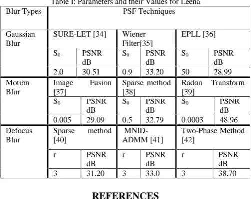
In this review paper the main purpose is to carry the comparative study for the restoration of blurred image. The different restoration algorithms used different types of parameters for their restoration purpose. The restoration is done in this review paper is based on the three types of blur like Gaussian blur, Motion blur, Defocus blur. These blurs are having the different parameters as standard deviation, radius and peak signal to noise ratio. Different restoration techniques has been developed and applied such as wiener filtering, multiscale-EPLL, fusion image deconvolution,
two phased method etc. Now a day’s graphical user
interface is used for the analysis of image restoration of blurred image.
Table I: Parameters and their Values for Leena
Blur Types PSF Techniques
Gaussian Blur
SURE-LET [34] Wiener Filter[35]
EPLL [36]
S0 PSNR
dB
S0 PSNR
dB
S0 PSNR
dB
2.0 30.51 0.9 33.20 50 28.99
Motion Blur
Image Fusion [37]
Sparse method [38]
Radon Transform [39]
S0 PSNR
dB
S0 PSNR
dB
S0 PSNR
dB
0.005 29.09 0.5 32.79 0.0003 48.96
Defocus Blur
Sparse method [40]
MNID-ADMM [41]
Two-Phase Method [42]
r PSNR
dB
r PSNR
dB
r PSNR
dB
3 31.20 3 33.0 3 38.70
REFERENCES
[1] Wei Hu, Jianru Xue and Nanning Zheng, “PSF via Gradient Domain Correlation”,IEEE Transaction on Image Processing, Vol. 21, No. 1, pp. 386-392, Jan. 2012.
[2] Feng Xue and Thierry Blue, “A Novel SURE-Based Criterian for
Parametric PSF estimation”, IEEE Transaction on Image Processing,
Vol. 24, No.2, pp. 595-607, Feb.2015.
[3] Rtnakar Dash, Pankaj Kumar Sa and Banshidhar majhi, “Particle
Swarm Optimization Based Support Vector Regression for Blind
Image Restoration”, Journal of Computer Science and Technology,
pp. 989-995, September 2012.
[4] Neel Joshi, Richard szeliski and Dayid J. Kriegman, “PSF estimation
using Sharp Edge Prediction” pp. 1-8, 2008.
[5] Haiyen CHEN, Minghua CAO, Huiqin WANG, Yan YAN and Lan
MA, “Estimation the Point Spread Function of Motion Blurred Images of the Ochotona Curzoniae”, International Congress in Image
and Signal Processing, Vol. 1, pp.369-373, 2013.
[6] Feng Xue and Thierry Blue, “A Novel SURE-Based Criterian for
Parametric PSF estimation”, IEEE Transaction on Image Processing,
Vol. 24, No. 2, pp. 595-607, February 2015.
[7] Wei Hu, Jianru Xue and Nanning Zheng, “PSF via Gradient Domain
Correlation”, IEEE Transaction on Image Processing, Vol. 21, No. 1,
pp. 386-392, January 2012.
[8] Feng- Qing Qin, Juin Min and Hong-Rong Guo, “A Blind Image Restoration Method Based on PSF Estimation”, IEEE World
Congress on Software Engg., Vol. 2, pp. 173-176, 2009.
[9] Chang-Hwan Son and Hyung-Min Park, “A Pair of Nosiy/blurry
Patches-based PSF Estimation and Channel-dependent Deblurring”,
IEEE Transaction on Consumer Electronics, Vol. 57, No. 4, pp. 1791-1799, November 2011.
[10] Shamik Tiwari, V. P. Shukla, and A. K. Singh, “Review of Motion Blur Estimation Techniques”, Journal of Image and Graphics, Vol. 1,
No. 4, pp. 176-184, December 2013.
[11] Feng-qing Qin, Jun Min and Hong-rong Guo, “A Blind Image restoration Method based on PSF Estimation”,World Congress on Software Engineering, Vol. 2, pp. 173-176, 19-21 May 2009. [12] Rajeshwari Natarajan, Govind S. Mudholkar, Michael P. Mc
Dermott, “Order restricted Inference for the Scale-Like Inverse
Gaussian Parametrs”, Elsevier Journal of Statistical Plannig and
Inferences, Vol.127, Issue 1-2, pp. 229-236, 1st January 2005. [13] Chris Stauffer, W.E.L Grimson, “Adaptive Background Mixture
Models for Real-Time Tracking”, IEEE Conference on Computer
Vision and Pattern Recognition, pp. 246-252, 23-25 June 1999. [14] Wang Taiyuel, LI Hongwei, LI Zhiming, Wang Zhihua, “A Fast
Parameter Estimation of Generalized Gaussian Distribution”,
International Conference on Signal Processing, Vol. 1, pp. 101-104, 2006.
[15] Jaskirat Singh and Sachin S. Sapatnekar, “A Scalable Statistical
Static timing Analyzer Incorporating Correlated Non Gaussian and
Gaussian Parameter Variations”, IEEE Transaction on CAD of IC
and Systems, Vol.27, No.1, pp. 160- 173, January 2008.
Gaussian Blur”, IEEE Transaction on Image Processing, Vol. 25,
No. 2, pp. 790-806, February 2016.
[17] Yang-Chih Lai, Chih-Li Huo, Yu-Hsiang Yu and Tsung-Ying Sun,
“PSO-Based Estimation for Gaussian Blur in Blind Image Deconvolution Problem”, IEEE Conference on Fuzzy Systems, pp.
1143-1148, 27-30 June 2011.
[18] Feng Xue, Thierry Blu, “Sure-Based Blind Gaussian
Deconvolution”, IEEE Statistical Signal Processing workshop, pp.
452-455, 5-8 August 2012.
[19] Haiyan CHEN, Minghua CAO, Huiqin WANG,Yan YAN and Lan
MA, “Estimation the Point Spread Function of motion-Blurred
Images of the Ochotona Curzoniae”, International Congress in Image
and Signal Processing, Vol. 1, pp. 369-373, 2013.
[20] Biswa Ranjan Mohapatra, Ansuman mishra, Sirat KumarRout, “A Comprehensive Review on Image Restoration Techniques”
International Journal of Research in Advent Technology, Vol. 2, No. 3, pp. 101-105, March 2014.
[21] Rui Xu, David Taubman and Aous Thabit Naman, “Motion
Estimation Based on Mutual Information and Adaptive Multi-Scale
Thresholding”, IEEE Transaction on Image processing, Vol. 25, No.
3, March 2016.
[22] Giacomo Boracchi and Alessandro Foi, “ Modeling the Performance of Image Restoration from Motion Blur”, IEEE Transaction on
image Processing, Vol. 21, No. 8, pp. 3502-3517, August 2012. [23] Caio-Kai Yu, Bing-Chen Tsai and Yin-Tsung Hwang, “An Efficient
Motion Blurred Image Restoration Scheme Based on Frequency
Domain Estimation”, IEEE Conference on Consumer Electronics,
pp. 1-2, 27-29 May 2016.
[24] Ratnakar Dash and Banshidhar Majhi, “ Motion Blur Parameters Estimation for Image Restoration”, Elsevier International Journal for
light and Electron Optics, Vol. 125, Issue 5, pp. 1634-1640, March 2014.
[25] Hujun Yin, “Blind Source Separation and Genetic Algorithm for
Image Restoration”, IEEE Conference on Advances in Space
Technology, pp. 167-172, 2-3 September 2006.
[26] Joao P. Oliveira, Mario A.T.Figueiredo, Jose M.Bioucas-Dias,
“Parametric Blur Estimation for Blind Restoration of Natural
Images: Linear Motion and Out-of-Focus”, IEEE Transaction on
Image Processing, Vol. 23, No. 1, pp. 466-477, January 2014. [27] Wikky Fawwaz A M, Takuya Shimahashi, Mitsuru Matsubara and
Sueo Sugimoto, “PSF Estimation and Image Restoration for Noiseless Motion Blurred Images”, ACM Conference on Signal, Speech and Image Processing, pp. 1-7, 15 July 2007.
[28] Ashwani M. Deshpande, Suprava Patnaik, “Radon Transform Based
Uniform and Non-Unifrom Motion Blur Parameter Estimation”,
IEEE Conference on Communication, Information & Computing Technology, pp. 1-6, 19-20 October 2012.
[29] Jianping Shi, Li Xu, Jiaya Jia, “Just Noticeable Defocus Blur Detection and Estiamtion”, IEEE Conference on Computer Vision
and Pattern Recognition, pp. 657-665, 7-12 June 2015.
[30] Hejin Cheong, Eunjung Chae, Eunsung Lee, Gwanghyun Jo and
joonki Paik, “ Fast Image Restoration for Spatially Varying Defocus Blur of Imaging Sensor”, MDPI Journal of Sensors, vol. 15, Issue 1,
pp. 880-898, 6 January 2015.
[31] Shaojie Zhuo and Terence Sim, “ Defocus Map Estimation from a Single image”, Elsevier Computer Analysis of Images and Patterns, Vol. 44, Issue 9, pp. 1852-1858, September 2011.
[32] Xian Zhu, Scott Cohen, Stephen Schiller and Peyman Milanfar, “ Estimating Spatially Varying Defocus blur from a Single Image”,
IEEE Transaction on Image Processing, Vol. 22, Issue 12, pp. 4879-4891, 21 August 2013.
[33] Elhusain Saad and Keigo Hirakawa, “ Defocus Blur-Invarient
Scale-Space Feature Extractions”, IEEE Transaction on Image Processing,
Vol. 25, No. 7, July 2016.
[34] Feng Xue and Thierry Blue, “A Novel SURE-Based Criterian for
Parametric PSF Estimation”, IEEE Transaction on Image Processing,
Vol. 24, No. 2, pp. 595-607, February 2015.
[35] Feng-qing Qin, Jun Min, Hong-rong Guo, “A Blind Image Restoration Method Based on PSF Estimation”,IEEE Conference on Software Engineering, Vol. 2, pp. 173-176, 2009.
[36] Vardan Papyan and Michael Elad, “Multi-Scale Patch-Based Image
Restoration”, IEEE Transaction on Image Processing, Vol. 25, No. 3,
pp. 249-261, January 2016.
[37] Mohini Sharma, Shilpa Datar, “Image Restoration Using Wavelet Based Image Fusion”, International Journal of Engineering Trends
and Technology, Vol. 15, No. 1, pp. 35-38, September 2014. [38] Ashwani M. Deshpande and Suprava Patnaik, “ Uniform and Non
-Uniform Singlre Image Deblurring based on Sparse representation
and Adaptive Dictionary Learning”, International Journal of
Multimedia and Its Applications, Vol. 6, No. 1, February 2014. [39] Anil Gupta, “Design and Analysis of Image Restoration Algorithm
using Radon Transform and Bilateral Filter”, International Journal of
Engineering and Management Research, Vol. 4, Issue 2, pp. 212-216, April 2014.
[40] Chia-Chen Lee and Wen-Liang Hwang, “Sparse representation of a Blur kernel for Blind Image Restoration”, ARXIV: 1512.04418v1,
pp. 1-9, 14 December 2015.
[41] Si Wnag, Ting-Zhu Huang, Xi-leZhao and Jun Liu, “An Alternating Direction Method for mixed Gaussian Plus Impulse Noise removal”,
Abstract and Applied Analysis, June 2013.
[42] Jian-Feng Cai, Raymond H. Chan, Mila Nikolova, “Two-Phase Approach for Deblurring Images Corrupted by Impulse plus
gaussian Noise”, Journal of Inverse Problems and Imaging, Vol. 2,
No. 2, pp. 187-204, 2008.
AUTHORS
Ritesh Pawar received the B.Tech degree in Electronics and communication from P.T.U, Jalandhar, India in 2010. He is pursuing his M.E in Electronics & Communication from
National Institute of Technical Teachers’
Training & Research Chandigarh India. His current research interests focus on Digital Signal Processing and Image Processing.