LARGE EDDY SIMULATION OF THE DIFFUSION PROCESS OF NUTRIENT-RICH UP-WELLED SEAWATER

LARGE EDDY SIMULATION OF THE DIFFUSION PROCESS OF

NUTRIENT-RICH UP-WELLED SEAWATER

Shigenao Maruyama

, Masud Behnia

, Masasazumi Chisaki

, Takuma Kogawa

a

Institute of Fluid Science, Tohoku University, Katahira, Aoba-ku, Sendai 980-8577, Japan

, Junnosuke Okajima

, and Atsuki

Komiya

b

School of Aerospace, Mechanical and Mechatronic Engineering, The University of Sydney, NSW 2006,Australia

c

School of Engineering, Tohoku University, Aoba 6-6, Aramaki-aza, Aoba-ku, Sendai 980-8579, Japan

A

The diffusion process of deep seawater drawn up by a vertical pipe deployed in the ocean is investigated. This vertical pipe is based on the principal of perpetual salt fountain. Numerical simulations of seawater upwelling from the pipe are performed based on experiments conducted in the Mariana trench region. Two turbulence modeling approaches were examined: k-ε model and Large Eddy Simulations (LES). The results in both models show that diffusion of the deep seawater diffusion after ejection from the pipe. The LES results show a 50% lower vertical penetration compared to the k-ε model as well as well as predicting that the horizontal diffusion is stronger than the vertical one.

Keywords: Perpetual salt fountain, Deep seawater, Nutrient transport, Eddy diffusion

* _{Corresponding author. Email: [email protected]}

1. INTRODUCTION

A rapid growth of world’s population has led to a need for more food, however an expansion of farm production has been somewhat limited. In contrast, there is a large ocean area which area that has not been used for food production. Increasing of food production in this area needs to be explored. The upwelling of deep seawater provides the euphotic surface layer with nutrients of deeper ocean, resulting in an increase in the oceanic productivity. A large area of the ocean, except some upwelling regions and high latitude domains, is characterized by a low productivity where low nutrient levels of the surface water prevent phytoplankton growth. Therefore, this large area does not play a role in supplying biological and fisheries resources.

Maruyama et al. (2004) have proposed a concept for increasing of food production by artificial upwelling of the deep seawater using a perpetual salt fountain (Stommel et al., 1956). Perpetual salt water fountain is a principle which allows bringing the deep seawater to the surface,(note that which “deep” seawater is defined as the seawater deeper than 200 m containing rich nutrients such as NO3 and PO4

Sunlight does not reach this depth, preventing phytoplankton from its photosynthesis and thus its growth. When a vertical pipe is deployed in the ocean where the hydrographic structure is characterized by a salinity minimum and filled with the deep seawater less saline than upper layers, the heating by outside warm water results in a buoyancy force leading to an upwelling flow in the pipe (see Fig. 1). Since this upward flow is accompanied with an uptake of less saline deep seawater into the pipe, the artificial upwelling is perpetually maintained. One of the advantages of this upwelling method is that it does not require any energy input except for the initial filling of the pipe with the deep seawater. This mechanism can be adopted in a large tropical and subtropical region where the minimum salinity layer is observed at depths of 300 to 600 m (Reid, 1965; Talley, 1993). This salinity

minimum is usually referred to as “intermediate water” in oceanography (Reid, 1965; Talley, 1993, 1999, 2003; Schmitz, 1995, 1996a, 1996b; Yasuda et al., 1996).

Fig. 1Schematic diagram of perpetual salt fountain

The upward flow in the vertical pipe deployed in the ocean was first observed in the experiments of Maruyama et al. (2004), demonstrating the theoretical study of Stommel et al. (1956). The experiments were conducted in the Mariana Trench region in the Pacific Ocean (location coordinates: 11.43°N, 142.42°E). Figure 1 shows the composite image of surface chlorophyll concentration around the upwelling pipe at the experiment in 2005. As shown in Fig. 1, it was observed that the chlorophyll concentration at the pipe outlet was about 100 times larger than that in the surrounding surface seawater (Maruyama et al., 2011, POPULAR SCIENCE, 2011). In addition, Maruyama et al. (2011), Zhang et al. (2004 and 2006) conducted the

Frontiers in Heat and Mass Transfer

numerical simulation inside the upwelling pipe and Maruyama et al.

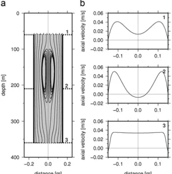
(2011) estimated upward flow velocity in the pipe was 2.45 mm/s (212 m/day). Similar values were also earlier obtained by Tsubaki et al. (2007). Figure 2(a),(b) show the simulated trajectories and simulated upwelling velocities in each depth (Maruyama et al. 2011). As shown in this Fig. 2, numerical simulation predicted the reverse flow at the central section of pipe. Zhang et al. (2004) predicted that the deep seawater descends 10 m after the ejection from the pipe outlet. In consideration of the practical use of the upwelling flow, one should focus on the nutrients, and its diffusion process from the pipe outlet to the ocean surface layers. It is known that in the ocean, turbulent diffusion is much larger than the molecular diffusion (Ledwell et al., 1998), therefore diffusion should be treated as turbulent diffusion in a numerical simulation.

Fig. 1 Composite image of surface chlorophyll concentration anomaly

around floating pipe system (Dots represent the grid at which signal is statistically significant level of 1%.) Maruyama et al. (2011)

Fig. 2 (a) Simulated trajectories and (b) simulated upwelling velocities

inside the pipe. The inside areas of the pipe are illustrated as the shaded area of (a). Upwelling velocities at 3 sections (1: outlet, 2: central section, 3: inlet) are shown. The location of 3 sections are labeled in (a). Maruyama et al. (2011)

In order to estimate the impact of the deep seawater fountain on increasing the oceanic productivity, it is necessary to predict the diffusion process of the deep seawater ejecting from the pipe outlet. Williamson et al. (2009) simulated the process of outflow from the pipe deployed in the Mariana trench by adopting a k-ε turbulence model (Launder and Spalding, 1973), which assumes isotropic turbulence viscosity. Their k-ε simulations were carried out with various turbulent Schmidt and Prandtl numbers. Their results showed that the horizontal advection is dominant in the diffusion process of the nutrients. However, turbulent Schmidt and Prandtl numbers had little effect on the results.

Further, they noted that the assumption of isotropic turbulence viscosity caused an overestimation of the vertical diffusion. The oceanic diffusivity is still a topic of contemporary oceanography, however, it is well-known that the horizontal diffusion is much larger than the vertical diffusion (Ledwell et al., 1998; Toole and McDougall, 2001). Therefore, this requires that in numerical simulations the turbulence anisotropy is taken into account. Hence, one could argue that the Direct Numerical Simulation (DNS) will be the best way to overcome this problem. Of course, DNS is computationally very expensive, in particular when both the spatial and temporal scales of the calculation is large, such as the present case.

Previously k-ε results have been shown not to reproduce the physical phenomena. Therefore in order to check and see if the turbulence model has been the cause of this discrepancy, a more sophisticated LES would have been tested. LES model (Smagorinsky, 1963; Liu et al., 1997; Yuan et al., 1999; Lewis, 2005) is a less computationally intensive approach than DNS. Here, we adopt an LES model for the simulation of the diffusion process of deep seawater after leaving the pipe outlet. In LES, it is assumed that, only the turbulence viscosity smaller than the grid scale (i.e. sub grid scale - SGS) is isotropic and the turbulence larger than the grid scale (GS) is directly simulated. Thus, LES may provide more realistic results and overcome some of the issues encountered when using a k-ε type model.

Recently, due to the advent of more powerful computers, LES has become a common tool to simulate turbulence in a variety of flow types. Of relevance is the study of Lewis (2005) who coupled LES with a model for plankton population dynamics to simulate the dispersion nutrients in the North Pacific. Liu et al. (1997) simulated a temperature stratified channel flow using LES, with taking into account the fluctuations due to the buoyancy force. Flöhlich et al. (2004) also used LES to simulate the turbulent flow around a cylinder (note: a similar geometry to our present study). However, their related cross-flow Reynolds number was much higher than that of present study. Yuan et al. (1999) simulated a round jet in cross-flow also by using LES. The performed their calculations at two Reynolds numbers, 1050 and 2100, which is close to the present study. Sun et al (2007) simulated buoyancy-driven convection in a rotating disk cavity using LES and unsteady Reynolds-Averaged Navier-Stokes (RANS) modeling, resulting in LES solution in better agreement with velocity and heat transfer measurements.

Very little LES work is published relevant to the oceanic environment which takes into account the temperature stratification and concentration fields in depths of 10–100 m. In this study, the diffusion process of outflow from the outlet of the vertical pipe deployed in the Mariana region is simulated by using LES. The objectives of this study are to investigate whether the behavior seen in oceans is observed using an LES model and to compare the LES results with the more commonly used k-ε turbulent model simulations.

2. GENERAL GUIDELINES

2.1 Governing Equations

In Large Eddy Simulation, the grid scale (GS) and sub-grid scale (SGS) are separated by filtering the Navier-Stokes equations as shown in Eqs. (1)–(4) below. Here, only the SGS turbulence is modeled, while GS turbulence is directly solved.

0,

i

i

u x

∂ ₌

∂ (1)

0 0

1

,

ref

i i i

j sgs ij i

j i j j

u u p u

u g

t x x x x

ρ ρ

ν τ

ρ ρ

   − 

∂ ₊ ∂ _{= −} ∂ ₊ ∂ ∂ _{− +}

   

 

∂ ∂ ∂ ∂ _ ∂ _{  } (2)

,

sgs j

j j t j

T T T

u

t x x Pr x

ν α

 

∂ ₊ ∂ ₌ ∂ ₊ ∂

 

,

sgs j

j j t j

C C C

u D

t x x Sc x

ν

 

∂ ₊ ∂ ₌ ∂ ₊ ∂

 

∂ ∂ ∂ _{ }∂ (4)

Where the bar represents the mean component for each variable. It should be emphasized that LES averaging is spatial based, whereas in k-ε type models a temporal or ensemble average is considered. The SGS stress component τij in Eq. (2) is expressed as follows,

1

2 ,

3

ij kk ij sgsSij

τ − τ δ = −ν (5)

Where the strain rate tensor

S

.

j i ij

j i

u u S

x x

∂ ∂

= +

∂ ∂ (6)

The SGS turbulent kinematic viscosity νsgs is obtained by using the standard Smagorinsky-Lilly model,

2

2 ,

sgs Lsgs S Sij ij

ν = (7)

Where the SGS mixing length Lsgs is obtained by using the following equation,

(

)

min , .

sgs s

L = κd C V (8)

The model constants used in our simulations were chosen as noted below.

s t t

C = 0.1, = 0.4187, Pr = 0.85, Sc = 0.7.κ (9)

These constant values have been tested and are known to apply to a wide range of flows (Launder et al., 1974; Yoshizawa et al., 1995, FLUENT, 2006) and were therefore chosen for the present simulations.

It should be noted that the SGS model in LES still assumes an isotropic turbulence. However, this is reasonable because the scale of the SGS turbulence is small enough to be treated as steady and isotropic in a statistical sense. Further, it is known that the large eddies of the GS affect most part of the solution and they primarily depend on the shape of the system and the boundary conditions, however the small eddies do not depend on the shape of the system and they can be treated as isotropic. Therefore, a general model can be obtained by modeling only the small eddies of the SGS. Further, since the spatial scale in this study is large, small eddies of the SGS are not expected to have much impact on obtaining an accurate numerical result.

2.2 Solution Method

The numerical simulation was conducted using a commercial CFD package (FLUENT 6.3). The governing equations were discretized using the second-order upwind scheme. An explicit time-advancement scheme with the fractional step method was employed.

The calculation model considered in this study is shown in Fig. 3. The domains dimensions are 17 m × 15 m × 6 m (see Fig. 2) and pipe diameter was 0.3 m, which is the actual pipe diameter in the Mariana trench region experiments of Maruyama et al. (2004). The pipe length used in their experiment was 300 m, though in order to focus on the pipe outlet, only the upper 10 m of the pipe is included in this domain. The grid was made to be finer near the pipe outlet with the finest scale being 0.015 m. The computational grid consisted of 324,420 elements.

For the initial and boundary conditions of temperature and salinity (note: Practical Salinity Scale is used here; see UNESCO [1981]), the experimentally measured profiles shown in Fig. 4 were used. The

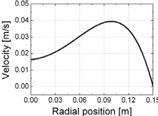
velocity boundary condition for the domain inlet was assumed to be a uniform and constant (0.015 m/s), which is the measured relative velocity between the pipe and the ocean flow. In addition we neglected the turbulent in inlet because the inlet velocity is very small. The outflow boundary condition was set as fully-developed. At the bottom of the pipe domain, the velocity profile shown in Fig. 5 was used. This velocity profile was based on the upwelling simulation results of Sato et al. (2007). For the nutrient, NO3 concentration at 300 m depth was

applied (Garcia et al., 2006). Other boundaries were set as a free-slip condition.

Fig. 3The computational model

Fig. 4 Vertical profiles of temperature and salinity in Mariana trench

region

Fig. 5Velocity profile employed for the bottom of the pipe domain

3. RESLUTS AND DISCUSSION

the k-ε model and 0.1 s for the LES. The concentration profile reached its steady state value at t = 10,000 s for the k-ε model and2,500 s for the LES.

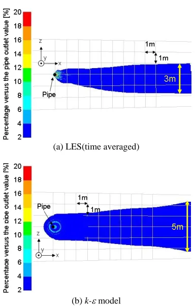
Figures 6 (a) and (b) show the cross-sectional view (along the x-y

plane) of nutrient contours for the LES and k-ε, respectively. Here, for comparison purposes and in order to clarify the differences, the time-averaged contours are shown for LES. The colored contours show the nutrient concentration percentages versus the distance.

Firstly, in order to show the effect of vertical diffusion, attention is drawn to the spread of the 2% contour level (see Fig. 6). It is noted that, downstream of the pipe outlet the predicted spreading width is 1 and 3 m for the LES and k-ε, respectively. Secondly, the 2% nutrient concentration contour level in the other direction (horizontal – top view) is examined. Here, the horizontal diffusion as shown in Figs. 7 (a) and (b) leads to a spread width of 3 and 5 m for the LES and k-ε, respectively. It should be noted that these figures are not the cross-sectional view at a certain depth, but the 2% nutrient concentration contour viewed from the top. Figures 7 (a) and (b) indicate that the ratio of the vertical diffusion to that of the horizontal one is about 33% for the LES, whereas in the case of the k-ε model it is about 50%.

As noted previously, the diffusion behavior seen in the ocean indicates that the horizontal diffusion is larger than the vertical one. The results here confirm that, at least as far as the ratio of the diffusion components is concerned, the LES results are more in line with the observations in the ocean.

The results here for both cases show that the nutrients ejected from the pipe descend downwards, and downstream of the pipe reach a neutral buoyancy. Furthermore, it is seen that the horizontal advection caused by the ocean flow is dominant, especially downstream of the pipe. The reason for the nutrient descent is that the salinity at the location (depth) of the pipe outlet is lower than that of the deep seawater ejected from the pipe outlet (see Fig. 4). However, as seen in Fig. 6 the vertical penetration of the two simulations is considerably different (i.e. 8 m for the k-ε model and 4 m for the LES).

In this calculation condition, there were some strong stratifications for temperature, salinity, nutrient. As stated in previous research (Filippo M. Denaro et al. 2007), the strong stratification with vertical direction makes the diffusion process with vertical direction anisotropic From the results presented here, it can be concluded that the k-ε model predicts a stronger diffusion (in both horizontal and vertical directions) than the LES. In the k-ε models, the flow was assumed isotropic with both vertical direction and horizontal direction and this model could not take into account the stratification effect. Because of this ignorance of stratification effect, the k-ε models predicted stronger diffusion with the vertical direction. Whereas, the LES model can directly simulate the flow and take into account the stratification effect at the resolved scale. Because of this reason, the calculation result of LES model showed the weaker diffusion with vertical direction compared to the k-ε modelas shown in Fig. 6 and it can be concluded that LES model qualitatively result can better represent the diffusion process than the k-ε model.

Of course, in order to ascertain this behavior quantitatively, future experiments to measure the nutrient concentrations are needed. Moreover, once the horizontal and vertical turbulent diffusion coefficients in the ocean are experimentally measured, then the LES model can be fine-tuned for better predictions. A strong diffusion of nutrients in the upstream direction is observed in Fig. 6(b). The k-ε model may over-predict the turbulent diffusion in the present flow situation. It is expected that the temporal average model may not be appropriate for simulation of the turbulent flow for the oceanic flow of the present scale.

In order to further examine the feasibility of a real perpetual salt fountain, future simulations need to focus on a larger scale of the order of 100 m. Of course, as the accuracy of the LES model depends on the grid size, the computational cost of such a large scale model may prove to be prohibitive. Further, the real ocean flow strongly affects the simulation results, however in the model used here a constant and uniform ocean flow was assumed. In fact, the ocean characteristics are

such that the flow direction and magnitude vary at all times. Introducing a more realistic ocean flow characteristics in the model will lead to more accurate results.

(a) LES(time averaged)

(b) k-ε model

Fig. 6 Nutrient concentration contours (cross-section view along x-y

plane)

(a) LES(time averaged)

(b) k-ε model

4. CONCLUDING REMARKS

In this study, we have performed turbulent flow simulations using the k -ε and LES models for a perpetual salt fountain. The diffusion process of the nutrient-rich deep seawater ejecting from a vertical pipe deployed in the ocean was numerically investigated. Based on the results obtained the following conclusions were reached.

(1) The LES model can qualitatively represent the behavior seen in real ocean compared to the k-ε model.

(2) A comparison of the LES and k-ε results show that the k-ε model predicts a stronger diffusion in both the horizontal and vertical directions.

(3) In order to quantitatively represent the real behavior seen in the ocean, future experiments to measure the nutrient concentrations as well as, horizontal and vertical turbulent diffusion coefficients are needed.

ACKNOWLEDGEMENTS

The calculations were conducted using the supercomputer SGI Altix at the Institute of Fluid Science, Tohoku University. This work was partially supported by a Grant-in-Aid for Scientific Research (B). The project was conducted collaboratively with Tokyo Metropolis.

NOMENCLATURE

C Concentration for salinity and nutrient (wt%)

Cs Smagorinsky constant (-)

D Distance from the wall (m)

d Molecular diffusion coefficient (m2s)

G Gravity acceleration (m/s2)

L Mixing length (m)

p Pressure (N/m2

Pr Prandtl number (-)

Sc Schmidt number (-)

ij

S Strain rate tensor (1/s)

t Time (s)

T Temperature (°C, K)

u Velocity (m/s)

V Cell volume (m3)

Greek symbols

α Thermal diffusivity (m2/s) δij Kronecker delta (-) κ Von Karman constant (-) ν Kinematic viscosity (m2/s) ρ Density (kg/m3)

τ Shear stress (m2_/s2₎

Subscripts

i, j, k Tensor index

ref Reference

sgs Sub grid scale

t Turbulent

x, y, z Coordinates 0 Ocean surface

REFERENCES

BONNIER corporation (2011): POPULAR SCIENCE May 2011.

FLUENT Inc. (2006): FLUENT6.3 User's Guide.

Filippo M. Denaro, Giuliano De Stefano, Daniele Iudicone, Vinecenzo Botte (2007): Afinite volume dynamic large-eddy simulation method for buoyancy driven turbulent geophysical flows. J Ocean Modeling, 17, 199-218.

http://dx.doi.org/10.1016/j.ocemod.2007.02.002

Fröhlich, J., W. Rodi, P. Kessler, S. Parpais, J. P. Bertoglio and D. Laurence (2004): Large eddy simulation of flow around circular cylinders on structured and unstructured grids. Notes on Numerical Fluid Mechanics, 66, 319–338.

Garcia, H.E., R. A. Locarnini, T. P. Boyer and J. I. Antonov (2006):World Ocean Atlas 2005, Volume 4: Nutrients (phosphate, nitrate, silicate), U.S. Government Printing Office.

Launder, B. E. and D. B. Spalding (1974): The numerical computation of turbulent flows. Computer Methods in Applied Mechanics and Engineering, 3, 269–289.

http://dx.doi.org/10.1016/0045-7825(74)90029-2

Ledwell, J. R., A. J. Watson and C. S. Law (1998): Mixing of a tracer in the pycnocline. J. Geophys. Res., 103, C10, 21499–21529.

http://dx.doi.org/10.1029/98JC01738

Lewis, D. M. (2005): A simple model of plankton population dynamics coupled with a LES of the surface mixed layer. Journal of Theoretical biology, 234, 565–591.

http://dx.doi.org/10.1016/j.jtbi.2004.12.013

Liu, N. Y., X. Y. Lu, S. W. Wang and L. X. Zhuang (1997): Large-eddy simulation of stratified channel flow. ActaMechanicaSinica, 13, 331– 338.

http://dx.doi.org/10.1007/BF02487192

Maruyama, S., K. Tsubaki, K. Taira and S. Sakai (2004): Artificial upwelling of deep seawater using the perpetual salt fountain for cultivation of ocean desert. J. Oceanogr., 60, 563–568.

http://dx.doi.org/10.1023/B:JOCE.0000038349.56399.09

Maruyama, S., T Yabuki, T. Sato, K. Tsubaki, A. Komiya, M. Watanabe, H. Kawamura and K. Tsukamoto (2011): Evidence of increasing primary production in the ocean by Stommel’s perpetual salt fountain, Deep-Sea Res. Part I-Oceanogr. Res. Pap., 58, 567–574.

http://dx.doi.org/10.1016/j.dsr.2011.02.012

Reid, J. L. (1965): Intermediate waters of Pacific Ocean, Johns Hopkins Oceanogr. Stud., 5, 96 pp.

Sato, T., S. Maruyama, A. Komiya and K. Tsubaki (2007):Numerical simulation of upwelling flow in pipe generated by perpetual salt fountain, Proceedings of16th Australian Fluid Mechanics Conference, 394–397.

Schmitz, W. J. (1995): On the interbasin-scale thermohaline circulation.

Rev. Geophys., 33, 151–173.

Schmitz, W. J. (1996a): On the world ocean circulation. Volume I, some global features/North Atlantic circulation, Woods Hole Oceanographic Institution, Technical Report, WHOI-96-03.

Schmitz, W. J. (1996b): On the world ocean circulation. Volume II, the Pacific and Indian Oceans/a global update, Woods Hole Oceanographic Institution, Technical Report, WHOI-96-08.

Smagorinsky, J. (1963): General Circulation Experiments with the Primitive Equations I, The basic experiment. Monthly Weather Review,

91, 99–164.

http://dx.doi.org/10.1175/1520-0493(1963)091%3C0099:GCEWTP%3E2.3.CO;2

Stommel, H., A. B. Arons and D. Blanchard (1956): An oceanographical curiosity: the perpetual salt fountain. Deep-Sea Res., 3, 152–153.

http://dx.doi.org/10.1016/0146-6313(56)90095-8

With a Central Axial Throughflow. J. Eng. Gas Turbines Power, 129, 318–325,

http://dx.doi.org/10.1115/1.2364192

Talley, L. D. (1993): Distribution and formation of North Pacific Intermediate Water. J. Phys. Oceanogr., 23, 517–537.

http://dx.doi.org/10.1175/1520-0485(1993)023<0517:DAFONP>2.0.CO;2

Talley, L. D. (1999): Some aspects of ocean heat transport by the shallow, intermediate and deep overturning circulations. p. 1–22. In Mechanisms of Global Climate Change at Millenial Time Scales,

Geophys.Mono. Ser. 112, ed. by P. U. Clark, R. S. Webb and L. D. Keigwin, American Geophysical Union

http://dx.doi.org/10.1029/GM112p0001.

Talley, L. D. (2003): Shallow, intermediate, and deep overturning components of the global heat budget. J. Phys. Oceanogr., 33, 530–560.

http://dx.doi.org/10.1175/1520-0485(2003)033<0530:SIADOC>2.0.CO;2

Toole, J. M. and T. J. McDougall (2001): Mixing and Stirring in the Ocean Interior. p. 337–355. In Ocean Circulation and Climate: Observing and Modelling the Global Ocean, ed. by G. Siedler, J. Church and J. Gould, Academic Press, San Diego.

Tsubaki, K., S. Maruyama, A. Komiya and H. Mitsugashira (2007): Continuous measurement of an artificial upwelling of deep sea water induced by the perpetual salt fountain. Deep-Sea Res. I, 54, 75–84.

http://dx.doi.org/10.1016/j.dsr.2006.10.002

UNESCO (1981): The Practical Salinity Scale 1978 and the International Equation of State of Seawater 1980, Unesco Technical Papers in Marine Science, 36, 25 pp.

Yasuda, I., K. Okuda and Y. Shimizu (1996): Distribution and modification of the North Pacific Intermediate Water in the Kuroshio-Oyashiointerfrontal zone. J. Phys. Oceanogr., 26, 448–465.

http://dx.doi.org/10.1175/1520-0485(1996)026<0448%3ADAMONP>2.0.CO%3B2

Yoshizawa, A., S. Murakami, T. Kobayashi, N. Taniguchi, Y. Dai, A. Kuroda, K. Kamemoto, S. Kato, Y. Nagano and T. Tsuji (1995):Analysis of Turbulent Flows, University of Tokyo Press., (in Japanese).

Yuan, L. L., R. L. Street and J. H. Ferziger (1999): Large-eddy simulations of a round jet in crossflow.Journal of Fluid Mechanics, 379, 71–104.

http://dx.doi.org/10.1017/S0022112098003346

Williamson, N., A. Komiya, S. Maruyama and M. Behnia (2009): Nutrient transport from an artificial upwelling of deep seawater. J. Oceanogr., 65, 349–359.

http://dx.doi.org/10.1007/s10872-009-0032-x

Zhang, X., S. Maruyama, S. Sakai, K. Tsubaki and M. Behnia (2004): Flow prediction in upwelling deep seawater — the perpetual salt fountain. Deep-Sea Res. I, 51, 1145–1157.

http://dx.doi.org/10.1016/j.dsr.2004.03.010

Zhang, X., S. Maruyama, K. Tsubaki, S. Sakai and M. Behnia (2006): Mechanism for enhanced diffusivity in the deep-sea perpetual salt fountain. J. Oceanogr., 62, 133–142.