R E S E A R C H A R T I C L E
Open Access
Outcome-sensitive multiple imputation:
a simulation study
Evangelos Kontopantelis
1,2*, Ian R. White
3, Matthew Sperrin
1and Iain Buchan
1Abstract
Background:Multiple imputation is frequently used to deal with missing data in healthcare research. Although it is known that the outcome should be included in the imputation model when imputing missing covariate values, it is not known whether it should be imputed. Similarly no clear recommendations exist on: the utility of incorporating a secondary outcome, if available, in the imputation model; the level of protection offered when data are missing not-at-random; the implications of the dataset size and missingness levels.
Methods:We used realistic assumptions to generate thousands of datasets across a broad spectrum of contexts: three mechanisms of missingness (completely at random; at random; not at random); varying extents of missingness (20–80% missing data); and different sample sizes (1,000 or 10,000 cases). For each context we quantified the performance of a complete case analysis and seven multiple imputation methods which deleted cases with missing outcome before imputation, after imputation or not at all; included or did not include the outcome in the imputation models; and included or did not include a secondary outcome in the imputation models. Methods were compared on mean absolute error, bias, coverage and power over 1,000 datasets for each scenario.
Results:Overall, there was very little to separate multiple imputation methods which included the outcome in the imputation model. Even when missingness was quite extensive, all multiple imputation approaches performed well. Incorporating a secondary outcome, moderately correlated with the outcome of interest, made very little difference. The dataset size and the extent of missingness affected performance, as expected. Multiple imputation methods protected less well against missingness not at random, but did offer some protection.
Conclusions:As long as the outcome is included in the imputation model, there are very small performance
differences between the possible multiple imputation approaches: no outcome imputation, imputation or imputation and deletion. All informative covariates, even with very high levels of missingness, should be included in the multiple imputation model. Multiple imputation offers some protection against a simple missing not at random mechanism.
Keywords:Multiple imputation, Imputed outcome, Missing data, Missingness
Background
Missing data is a common obstacle to observational health science and its pitfalls are well known [1]. To exclude study subjects with any missing covariate observa-tions, so called complete case analysis, is at best of low statistical power and at worst provides biased estimates.
The complexity of the missing data problem, or obtaining accurate inferential estimates in the presence
of missing data, depends on the nature of the mechan-ism by which data are missing [2]. The less problematic scenario occurs when the probability of an observable data point being missing (the missingness probability) does not depend on any observed or unobserved param-eters, and this missingness mechanism is known as Missing Completely at Random (MCAR). However, MCAR mechanisms are considered rare in practice, es-pecially for surveys [3]. More commonly, the missing-ness probability depends on observed variables, and hence it can be accounted for by the information con-tained in the dataset. This missing data mechanism has been labelled Missing at Random (MAR). Finally, the * Correspondence:[email protected]
1
The Farr Institute for Health Informatics Research, University of Manchester, Vaughan House, Manchester M13 9GB, UK
2NIHR School for Primary Care Research, Centre for Primary Care, Institute of Population Health, University of Manchester, Manchester, UK
Full list of author information is available at the end of the article
most challenging missingness mechanism occurs when the missingness probability depends on unobserved values, and called Missing Not at Random (MNAR). Using self-reporting of sexual activity we can explore MAR and MNAR examples. A MAR scenario would arise if girls are less likely than boys to report whether they are sexually active, but sexually active teenagers are no more likely to report than those non-active. However, if sexually active girls are less likely to report than non-active girls, this would be an MNAR scenario.
Although suboptimal approaches to imputation are still routinely used [4], multiple imputation has been ac-cepted by methodologists as the most appropriate framework for dealing with MCAR and MAR mecha-nisms [5]. Multiple imputation can be described in three steps: (a) drawing the missing data from their posterior predictive distribution under a posited Bayesian model, across N datasets; (b) analysing each dataset separately with a chosen method, usually a regression model; and (c) pooling the estimates and their standard errors across the N analyses using Rubin’s rules [2], allowing for the use of the within-imputation and between-estimation variation components in the calculations. Multiple im-putation has a largely Bayesian rationale but it also works well in frequentist applications by providing nom-inal coverage levels and unbiased point estimates [2]. When the analysis model (Step 2) is Bayesian the result-ing framework is fully Bayesian; alternatively, frequentist maximum-likelihood estimates can be used in the model to draw missing values [6, 7]. An interesting trait of mul-tiple imputation is that it performs better at imputing missing predictors when outcome information is in-cluded in the models [8]. Although standard applications of multiple imputation do not deal with MNAR mecha-nisms, they can offer some protection against them [9]. Furthermore, multiple imputation can accommodate MNAR scenarios flexibly and is thus well-suited to sen-sitivity analyses [10].
This paper tackles five outstanding issues about mul-tiple imputation. von Hippel argued that researchers should impute values for the outcome, but exclude cases with imputed outcomes when fitting the substantive model [11]. It is unclear when this is the best strategy compared with not imputing the outcome on the one hand, and using imputed outcomes in the analysis on the other hand.
Another question of practical interest is how much missingness should be considered manageable within a multiple imputation framework, i.e. is the performance of multiple imputation consistent as missingness in-creases and is there a level above which performance de-teriorates to such an extent that it makes the method and data of little practical use? Although this has been answered for multiple imputation that does not impute
the outcome, which was found to perform consistently across all missingness levels [12], the question remains for outcome imputations.
Also unknown is the role of multiple correlated out-comes in the imputation models. It is not uncommon for studies to collect information on two or more corre-lated outcomes. However, these outcomes are often ana-lysed through separate multiple imputation models, which do not utilise the association of the outcome of interest with a second (or more) available outcome. Would the inclusion of a second outcome lead to an im-proved multiple imputation model?
In addition, as far as we know, the level of protection, if any, offered by current multiple imputation methods (i.e. methods that assume MAR) against MNAR mecha-nisms has not been quantified within a simulations framework. Although there are technical challenges and numerous assumptions when developing such a frame-work, a high level of protection would make researchers more confident when reporting results from analyses with missing data—especially since MNAR mechanisms cannot be identified without additional external data or prior knowledge.
Finally, the size of the investigated dataset could be an important parameter and the performance of multiple imputation has largely been assessed in small or moder-ate datasets [8, 13], mainly for computational reasons. We have chosen scenarios of 1000 cases, which would be relevant to small and moderate studies, and more or less in agreement with previous investigations. However, it is now common to analyse data from many thousands or even millions of people, for example using Electronic Health Records (EHRs), and for this reason we also ana-lysed scenarios of 10,000 cases.
In this paper we address all of the questions above using simulations. We simulate a wide range of scenarios which are not uncommon in observational studies with databases of routinely collected data, where hundreds of variables may be available and often have varying levels of missingness [14]. Although our motivation stems from our experiences with observational data, our find-ings are also relevant to clinical trials data, which are usually less variable (e.g. levels of missingness across var-iables are uniform, when someone is lost to follow-up).
Methods
were repeated 1,000 times, to obtain different datasets under the specified parameters and to analyse them.
Data generation
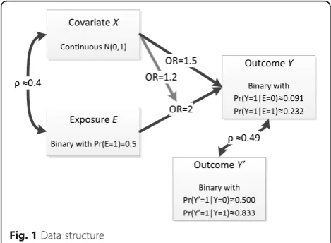
We assumed two dataset sizes of 1,000 and 10,000 patients for which we originally had complete information on a pri-mary binary outcomeY, a secondary binary outcomeY’, a binary exposure variable E and a continuous covariate X confounding the relationship between exposure and out-comes. The whole process was implemented in Stata v14.1 [15], and the code is provided in Online Additional file 1. We used the drawnorm command to draw observations from multivariate normal distributions, allowing for a≈0.4 Pearson’s correlation between X and E. Covariate X had mean 0 and variance 1, while we set Pr (E= 1) = 0.5. Out-come Y’was generated last, correlated with primary out-comeY(tetrachoricρ≈0.49), but independent ofXandE givenY. Writingπ=p(Y= 1|X,E), we assumed the logistic regression model logit(π) =β0+β1E+β2X+β3E⋅X with parameters: exp (β0)≈0.091, exp (β1) = 2, exp (β2) = 1.5 and exp (β3) = 1.2. These parameters lead to conditional probabilities for the outcome of Pr (Y= 1|E= 0) = 0.091 and Pr (Y= 1|E= 1) = 0.232. Weaker associations exist be-tweenY’andE,Y’andX,Y’andX*E, but are not of inter-est. The data structure is displayed in Fig. 1.
Missingness mechanisms
We implemented three missing data mechanisms (MCAR, MAR and MNAR) and four levels of overall missingness for each variable (20%, 40%, 60% and 80%). In each case, covariate Xand outcomes YandY’all had the same level of missingness but information for expos-ureEwas always complete. In the MCAR setting, values for X,YandY’were independently set to be missing. In the MAR setting, the probability to be missing for each ofX,YorY’was independently set to be conditional on the exposure EwithOR= 5. In other words, the odds of a missing value for X,Yor Y’were five times as high in
the presence of the exposure (i.e. when E= 1). In the final setting, a relatively simple MNAR scenario, the probabilities of missing data for X,Yor Y’ were condi-tional on the true values ofX,Yor Y’respectively, with OR= 5 used across each of the associations. Information for exposure E was always complete. However, the MNAR scenario is of course not exhaustive and alterna-tive MNAR mechanisms could vary across exposure groups [16]. It should also be noted that although the missingness mechanism we modelled is rather extreme, it was a conscious decision to make it more likely to ob-serve performance variability across models. We antici-pate our findings to be relevant to weaker associations, where model performances are expected be less variable.
Alternative data structures
We also considered two alternative structures, as sensi-tivity analyses, which we do not present in detail in this paper but the code for which is available from the authors. In the first sensitivity analysis we simulated a continuous rather than a binary outcome, and in the sec-ond sensitivity analysis we included a secsec-ond covariateX’ to which we applied the same missingness mechanisms.
Analysis
Across each missingness mechanism we followed the same seven logistic regression analyses, seven of which were multiple imputation approaches (Table 1). The first analysis (A) was the simplest, a complete cases analysis, with the sole purpose of providing a benchmark against which to compare the multiple imputation approaches. In the remaining seven analyses we used the mi family of commands in Stata, with mi impute chained for the imputation and mi estimate with a multiple logistic re-gression (logitcommand) for the analysis. Analyses B, C, D and E all ignored the secondary outcome Y’. In the second analysis (B), which is known to give biased esti-mates [11], we excluded cases where the outcome was missing and the outcome was not included in the
Fig. 1Data structure
Table 1Analysis methods
A complete case analysis (no multiple imputation [mi]) B no outcome imputation, not included in mi model Ca no outcome imputation, outcome imputed in mi model Da outcome imputed and included in mi model
Ea outcome imputed and included in mi model but then cases where it was imputed are deleted
Fa as in C but also including a second correlated outcome in the mi model
Ga as in D but also including a second correlated outcome in the mi model
H as in D but the mi and analysis models do not include the covariate
a
imputation model. In the third analysis (C), we again dropped missing outcome cases but included the out-come in the imputation model for the missing covariate X. In the fourth analysis (D) we included the outcome in the imputation model and imputed its missing values as well as missing values for X. An alternative approach suggested by von Hippel [11] was our analysis E, which followed D and included the outcome in the multiple imputation model and imputing it, but deleted cases where the outcome was imputed. Analyses F and G, followed C and D respectively but also included the sec-ond outcome in the imputation models and imputed their missing values. Finally, analysis H followed the setup of D, except it did not include the covariate X in the multiple imputation or analysis models. This aimed to assess whether the covariate should be included, even when its missingness levels were very high.
The analysis approaches and the data setup were se-lected to fit our research questions. Comparing analysis models C and D, which are the commonly recom-mended best practice models, will provide information on whether imputing an incomplete outcome is prefera-ble to excluding the relevant cases. Model E, which deletes cases where the outcome is imputed, will be assessed as a best practice alternative to C and D. Com-parisons between C and F, as well as D and G will inform us whether the inclusion of a second outcome which is correlated to our outcome of interest leads to a better multiple imputation model. Comparing models that have included the covariate (e.g. C and D) with model H, across various levels of missingness, will an-swer whether it is preferable to exclude a covariate from a multiple imputation model when most of its values are missing. Simulating different missingness mechanisms will allow us to quantify the performance of multiple im-putation approaches vs complete case analyses in the most problematic MNAR scenario, compared to the known protection it offers for the most common MCAR and MCAR scenarios [13]. Finally, repeating the analyses in datasets of different sizes will shed light to whether our conclusions are sample-size dependent or not.
Performance measures
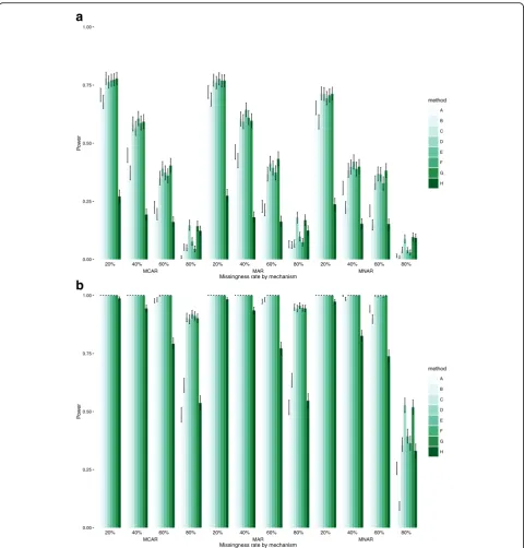
We aimed to measure the performance of all multiple imputation and analysis approaches with logistic regres-sion, across the scenarios of missingness described above and over 1,000 iterations, in the estimation of the three true association of interest:E→OR=2Y(our main focus), X→OR=1.5Y and X*E→OR=1.2Y. There are numerous performance measures that can be used in simulation studies [17], but we considered mean absolute error, mean bias, coverage probability and power of the ana-lyses in relation to the three parameters of interest to be adequate for our investigation. Mean absolute error was
calculated as 1 1000
X i¼1 1000
jz−zbijwherezis one of the three parameters of interest, expressed as a log-odds ratio. Analogously mean bias is the mean difference in the estimate to the true parameter, and was calculated as
1 1000
X i¼1 1000
ðz−zbiÞ. Therefore, assuming the used exposure effect of log[2], a reported mean bias of 0.1 or −0.1 would mean that the returned estimate was on aver-age≈log(1.81) or≈log(2.21), respectively. The coverage probability, is the proportion of 95% confidence inter-vals for the estimate that contain the true parameter across the 1,000 iterations. Theoretically this should be close to 95% but the bias introduced through the MAR and MNAR mechanisms can affect coverage levels. Fi-nally, we calculated the power to detect that the param-eter is different from zero by computing the proportion of the 1,000 95% confidence intervals for each param-eter that did not include zero. However, power needs to be carefully interpreted in the presence of bias since bias will move the estimate closer or further away from the alternative hypothesis on which power is calculated, and in the latter case higher bias will lead to higher power. Nevertheless, provided bias is similar across the methods to compare, power can be used for compari-sons, even if bias is not zero, and we felt it was an im-portant metric that would complement the study.
Results
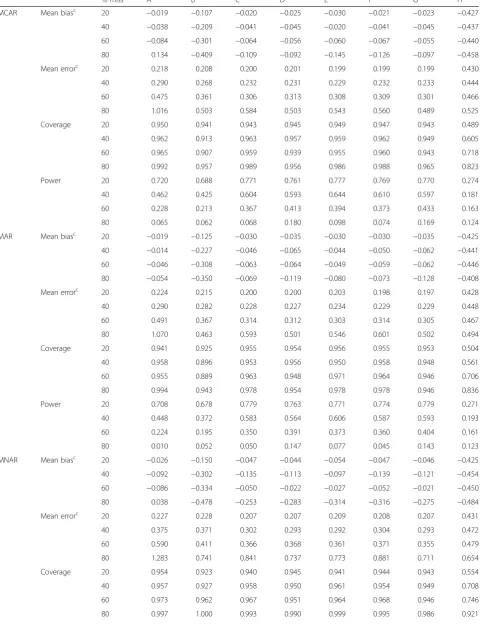
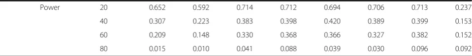
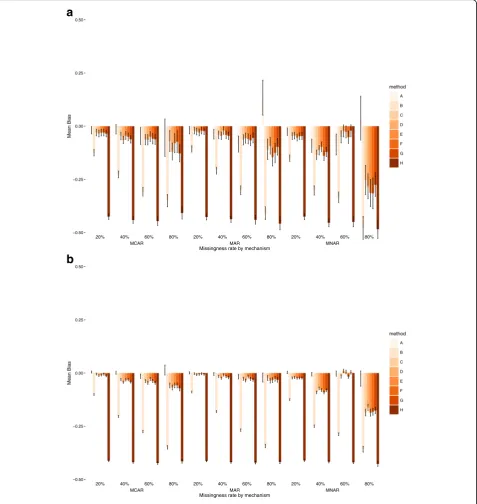
Results for the coefficient of the exposure β1 are pre-sented in Table 2 and Table 3 for datasets of 1,000 and 10,000 cases, respectively. Figures 2, 3, 4 and 5 present the exposure performance metrics with their respective error bars. Although all methods successfully converged for the larger datasets, there was some variation in the smaller datasets for very high levels of missingness (Online Additional file 2: Table S5). Results for the coefficients of the covariate and the exposure-covariate interaction are also presented in Online Additional file 2: Table S1, S2, S3 and S4).
Mean bias
Table 2Performance results for exposure E, datasets of 1,000 observationsa
% miss A B Cb Db Eb Fb Gb H
MCAR Mean biasc 20 −0.019 −0.107 −0.020 −0.025 −0.030 −0.021 −0.023 −0.427
40 −0.038 −0.209 −0.041 −0.045 −0.020 −0.041 −0.045 −0.437
60 −0.084 −0.301 −0.064 −0.056 −0.060 −0.067 −0.055 −0.440
80 0.134 −0.409 −0.109 −0.092 −0.145 −0.126 −0.097 −0.458
Mean errorc 20 0.218 0.208 0.200 0.201 0.199 0.199 0.199 0.430
40 0.290 0.268 0.232 0.231 0.229 0.232 0.233 0.444
60 0.475 0.361 0.306 0.313 0.308 0.309 0.301 0.466
80 1.016 0.503 0.584 0.503 0.543 0.560 0.489 0.525
Coverage 20 0.950 0.941 0.943 0.945 0.949 0.947 0.943 0.489
40 0.962 0.913 0.963 0.957 0.959 0.962 0.949 0.605
60 0.965 0.907 0.959 0.939 0.955 0.960 0.943 0.718
80 0.992 0.957 0.989 0.956 0.986 0.988 0.965 0.823
Power 20 0.720 0.688 0.771 0.761 0.777 0.769 0.770 0.274
40 0.462 0.425 0.604 0.593 0.644 0.610 0.597 0.181
60 0.228 0.213 0.367 0.413 0.394 0.373 0.433 0.163
80 0.065 0.062 0.068 0.180 0.098 0.074 0.169 0.124
MAR Mean biasc
20 −0.019 −0.125 −0.030 −0.035 −0.030 −0.030 −0.035 −0.425
40 −0.014 −0.227 −0.046 −0.065 −0.044 −0.050 −0.062 −0.441
60 −0.046 −0.308 −0.063 −0.064 −0.049 −0.059 −0.062 −0.446
80 −0.054 −0.350 −0.069 −0.119 −0.080 −0.073 −0.128 −0.408
Mean errorc 20 0.224 0.215 0.200 0.200 0.203 0.198 0.197 0.428
40 0.290 0.282 0.228 0.227 0.234 0.229 0.229 0.448
60 0.491 0.367 0.314 0.312 0.303 0.314 0.305 0.467
80 1.070 0.463 0.593 0.501 0.546 0.601 0.502 0.494
Coverage 20 0.941 0.925 0.955 0.954 0.956 0.955 0.953 0.504
40 0.958 0.896 0.953 0.956 0.950 0.958 0.948 0.561
60 0.955 0.889 0.963 0.948 0.971 0.964 0.946 0.706
80 0.994 0.943 0.978 0.954 0.978 0.978 0.946 0.836
Power 20 0.708 0.678 0.779 0.763 0.771 0.774 0.779 0.271
40 0.448 0.372 0.583 0.564 0.606 0.587 0.593 0.193
60 0.224 0.195 0.350 0.391 0.373 0.360 0.404 0.161
80 0.010 0.052 0.050 0.147 0.077 0.045 0.143 0.123
MNAR Mean biasc
20 −0.026 −0.150 −0.047 −0.044 −0.054 −0.047 −0.046 −0.425
40 −0.092 −0.302 −0.135 −0.113 −0.097 −0.139 −0.121 −0.454
60 −0.086 −0.334 −0.050 −0.022 −0.027 −0.052 −0.021 −0.450
80 0.038 −0.478 −0.253 −0.283 −0.314 −0.316 −0.275 −0.484
Mean errorc 20 0.227 0.228 0.207 0.207 0.209 0.208 0.207 0.431
40 0.375 0.371 0.302 0.293 0.292 0.304 0.293 0.472
60 0.590 0.411 0.366 0.368 0.361 0.371 0.355 0.479
80 1.283 0.741 0.841 0.737 0.773 0.881 0.711 0.654
Coverage 20 0.954 0.923 0.940 0.945 0.941 0.944 0.943 0.554
40 0.957 0.927 0.958 0.950 0.961 0.954 0.949 0.708
60 0.973 0.962 0.967 0.951 0.964 0.968 0.946 0.746
analysis appeared to be by the best performer with very low bias in every simulation scenario.
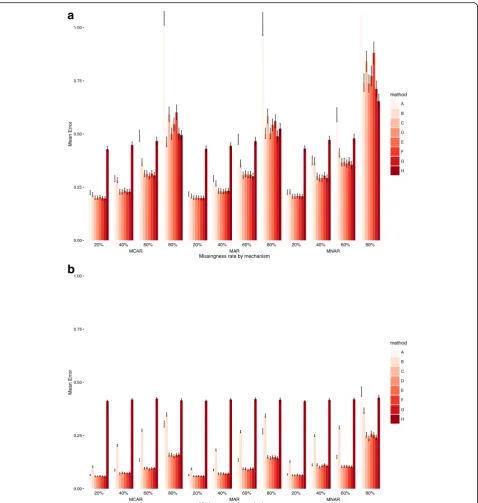
Mean absolute error
In both smaller and larger datasets, the best performing models were: C (no outcome imputation, outcome in-cluded in mi model); D (outcome imputed and inin-cluded in mi model); E (outcome imputed and included in mi model and then deleted); F (no outcome imputation, both outcomes included in mi model); and G (both outcomes included in mi model, outcome of interest imputed). For the smaller datasets, the models that imputed the out-come (D, E and G) generally performed only slightly better for very high levels of missingness in MCAR data, and for MAR data (and especially for higher rates of missingness). Error increased with increasing missingness but was not too dissimilar across the three missingness mechanisms. In the larger datasets, levels of mean absolute error were much lower and there was no benefit in using the second outcome, with models C, D and E performing the best, with variations in different settings. Overall, the best model was E but only slightly better than C and D.
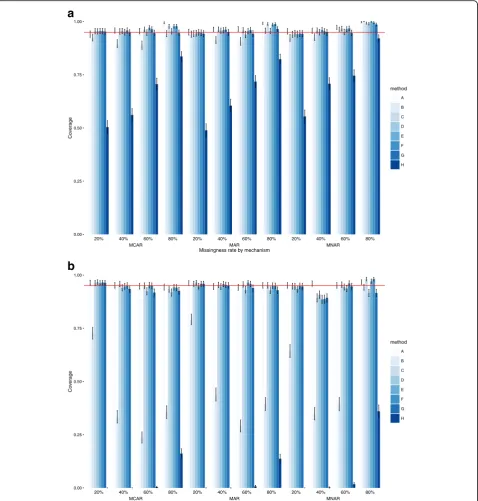
Coverage
Again, at both dataset sizes, models C, D, E, F and G per-formed best. There was very little to separate them, how-ever, the models that imputed the outcome (D and G) tended to be closer to the nominal 95%. There were rela-tively small differences across missingness mechanisms and coverage levels were good in all scenarios, with the lowest rates amongst the five top performing models observed for D and G in MAR data and high missingness levels. Simi-larly, coverage rates were consistently high across all levels of missingness. In larger datasets, there was no benefit to using a second outcome, with models C, D and E equiva-lent in almost all missingness scenarios. Overall, differences between models C, D and E are small but E had better coverage in the larger datasets for extensive missingness.
Power
Results for power were consistent with error and coverage, with models C, D, E, F and G again performing best. In
the smaller datasets, there were small differences between these models, except for very high levels of missingness, and especially for MCAR and MAR mechanisms, where imputing the outcome (models D and G) returned higher power level, albeit still very low. However, for lower levels of missingness, model C performed well and, more often than not, slightly better than D. The nature of the missing-ness mechanism had some effect on power, with lower levels observed for MNAR data, especially as levels of missingness increased. As expected, the more data are missing the lower the power, and all models performed very poorly for high or very high levels of missingness (60% or above). In larger datasets, the picture did not change with models C, D, E, F and G being almost equivalent, but model D performed better for extensive missingness (60% or above) in MNAR data. Overall, E out-performed C is all settings and D for low and moderate levels of missingness, while D performed better for very high levels of missingness.
Sensitivity analyses
Patterns of results in the two sets of sensitivity simula-tions broadly agreed with what we observed for the main simulations and further supported our findings. When analysing a continuous outcome, differences between multiple imputation models were again very small. Fo-cusing on datasets of 1000 observations and the multiple imputation models of main interest (C to G), mean bias was very similar for all missingness mechanisms and levels. Mean bias was very close to zero for all MCAR and MAR settings, except for 80% levels of missingness. For MNAR data, mean bias was very close to zero for 20% missingness and linearly increased with missingness. Mean absolute error was again similar in these methods across all missingness mechanisms, with some variability being observed for 80% missingness and method G (out-come imputed and included in mi model, including sec-ondary outcome) performing slightly better in those scenarios (Online Additional file 2: Figure S1). Coverage was similar in all scenarios, except for high levels of missingness where the outcome imputation models (G and especially D) slightly underperformed. However, that
Table 2Performance results for exposure E, datasets of 1,000 observationsa(Continued)
Power 20 0.652 0.592 0.714 0.712 0.694 0.706 0.713 0.237
40 0.307 0.223 0.383 0.398 0.420 0.389 0.399 0.153
60 0.209 0.148 0.330 0.368 0.366 0.327 0.382 0.152
80 0.015 0.010 0.041 0.088 0.039 0.030 0.096 0.092
a
Analysis model A: complete case analysis (no multiple imputation [mi]); B: no outcome imputation, not included in mi model; C: no outcome imputation, outcome imputed in mi model; D: outcome imputed and included in mi model; E: outcome imputed and included in mi model but then observations where it was imputed are deleted; F as in C but also including a second correlated outcome in the mi model; G as in D but also including a second correlated outcome in the mi model; H as in D but the mi and analysis models do not include the covariate
b
Main models of interest, other models provided for comparison purposes
c
Table 3Performance results for exposure E, datasets of 10,000 observationsa
% miss A B Cb Db Eb Fb Gb H
MCAR Mean biasc 20 0.001 −0.089 −0.003 −0.008 −0.006 −0.003 −0.006 −0.413
40 −0.005 −0.181 −0.016 −0.024 −0.009 −0.016 −0.021 −0.419
60 −0.017 −0.268 −0.027 −0.035 −0.017 −0.028 −0.032 −0.421
80 −0.021 −0.343 −0.023 −0.036 −0.033 −0.027 −0.032 −0.418
Mean errorc 20 0.064 0.094 0.059 0.059 0.060 0.059 0.059 0.413
40 0.088 0.182 0.071 0.072 0.071 0.070 0.071 0.419
60 0.135 0.268 0.094 0.094 0.088 0.094 0.095 0.421
80 0.270 0.343 0.150 0.144 0.148 0.148 0.143 0.418
Coverage 20 0.962 0.792 0.959 0.965 0.948 0.959 0.959 0.000
40 0.946 0.439 0.954 0.946 0.958 0.954 0.952 0.000
60 0.943 0.291 0.956 0.931 0.965 0.958 0.939 0.007
80 0.952 0.394 0.952 0.929 0.950 0.949 0.929 0.137
Power 20 1.000 1.000 1.000 1.000 1.000 1.000 1.000 0.983
40 1.000 1.000 1.000 1.000 1.000 1.000 1.000 0.935
60 0.974 0.982 1.000 1.000 1.000 1.000 1.000 0.772
80 0.518 0.635 0.949 0.943 0.956 0.946 0.944 0.547
MAR Mean biasc
20 0.005 −0.101 −0.005 −0.012 −0.009 −0.005 −0.013 −0.412
40 0.001 −0.204 −0.031 −0.043 −0.032 −0.031 −0.042 −0.419
60 −0.015 −0.275 −0.038 −0.046 −0.028 −0.037 −0.046 −0.423
80 0.014 −0.349 −0.058 −0.068 −0.058 −0.058 −0.072 −0.415
Mean errorc 20 0.064 0.104 0.059 0.058 0.060 0.058 0.058 0.412
40 0.087 0.204 0.072 0.075 0.074 0.072 0.075 0.419
60 0.135 0.275 0.096 0.098 0.092 0.095 0.097 0.423
80 0.304 0.349 0.160 0.159 0.153 0.158 0.161 0.415
Coverage 20 0.965 0.727 0.963 0.967 0.962 0.965 0.964 0.000
40 0.952 0.334 0.958 0.940 0.947 0.951 0.935 0.000
60 0.948 0.237 0.950 0.924 0.953 0.950 0.918 0.004
80 0.944 0.356 0.935 0.918 0.943 0.941 0.926 0.161
Power 20 1.000 1.000 1.000 1.000 1.000 1.000 1.000 0.987
40 1.000 1.000 1.000 1.000 1.000 1.000 1.000 0.944
60 0.977 0.982 0.999 1.000 1.000 1.000 1.000 0.792
80 0.486 0.613 0.905 0.897 0.920 0.912 0.902 0.537
MNAR Mean biasc
20 0.003 −0.125 −0.023 −0.021 −0.024 −0.023 −0.024 −0.411
40 −0.006 −0.250 −0.091 −0.072 −0.080 −0.091 −0.081 −0.417
60 −0.003 −0.288 −0.016 0.010 0.005 −0.017 0.003 −0.420
80 −0.026 −0.358 −0.186 −0.161 −0.186 −0.182 −0.176 −0.427
Mean errorc 20 0.067 0.128 0.063 0.063 0.066 0.063 0.063 0.411
40 0.112 0.250 0.113 0.102 0.107 0.113 0.107 0.417
60 0.150 0.288 0.103 0.105 0.106 0.104 0.103 0.420
80 0.456 0.367 0.253 0.237 0.258 0.252 0.241 0.428
Coverage 20 0.952 0.643 0.948 0.947 0.935 0.949 0.947 0.000
40 0.960 0.349 0.893 0.908 0.886 0.887 0.893 0.002
60 0.952 0.394 0.955 0.944 0.937 0.961 0.947 0.017
shortcoming was counterbalanced for model G by higher power in all scenarios except very low levels of missing-ness, where there was very little variation in perform-ance (Online Additional file 2: Figure S2).
Discussion
Our results indicate that in general, there are very small differences between models that impute the outcome compared with those that do not, when all else is equal and the outcome is included in the imputation model. However, in some contexts small differences emerge that should underpin recommendations as to the choice of model. The von Hippel approach [11], our model E, where the outcome is included in the imputation model and imputed but cases where the outcome is imputed are later dropped performed well. However, the differ-ences between this approach and alternative models, where the outcome is not imputed or imputed and not dropped, were generally very small if any (error bars for all performance metrics overlapped substantially). Fur-thermore, the von Hippel approach was not consistently better in all scenarios. Another consideration is the pres-ence of an“auxiliary”variable, a variable that in not part of the analysis model but is used in the multiple imput-ation to improve the prediction of missing values. If such a variable is associated with missingness in the out-come, model E is known to produce biased parameter estimates and should be avoided [18].
The level of missingness naturally affects the perform-ance of the multiple imputation models, especially with regards to power (primarily) and error (secondarily). However, in agreement with Janssen et al. [12], we rec-ommend using all available data even when missingness among covariates of interest is extensive. Multiple im-putation models that exclude such covariates seem to perform much worse. For very high levels of missingness and moderately sized datasets we recommend the use of simulation-based platforms to estimate the power to de-tect effects [19]. Convergence was not an issue with any models when the datasets contained 10,000 observa-tions, but it was a factor to consider in the 1,000
observations datasets as the level of missingness in-creased. Multiple imputation models that did not impute the outcome and were only modestly affected, while complete case analysis was severely affected.
The size of the datasets (1,000 or 10,000) did not sub-stantially affect how the models ranked within each group. Interestingly, in the larger datasets, a complete case ana-lysis approach was generally only slightly worse than the best performing multiple imputation models for low levels of missingness. Therefore, existing multiple imputation approaches may be less relevant to large health informat-ics databases than to randomised clinical trials.
Surprisingly the inclusion of a second outcome in the multiple imputation model, moderately correlated to the primary outcome, made very little difference to perform-ance. Since for the imputation model there is no real distinction between predictors and outcomes, we would expect the inclusion of the secondary outcome to lead to improved performance. However, our findings could be explained by the associations between the predictors and the secondary outcome. In other words, the secondary outcome has little independent information to add to the model. A weaker association between predictors and secondary outcomes and a stronger correlation between outcomes would make the secondary outcome a useful addition to the multiple imputation model. However, we did observe slightly better performance for the model in the continuous outcome sensitivity analysis, for some scenarios, mainly in terms of power but also mean abso-lute error. Hence a more complete multiple imputation model that includes all outcomes is recommended.
Finally, although all models performed worse when data were MNAR, multiple imputation models can offer some protection, in terms of mean absolute error, even in this relatively extreme missingness scenario we simu-lated (OR = 5 for the missingness mechanism). Multiple imputation models outperformed complete case analyses in both smaller and larger datasets. However, the bene-fits of using multiple imputation methods were not as high for MNAR as for MCAR or MAR data, and were more obvious in the smaller datasets.
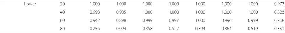
Table 3Performance results for exposure E, datasets of 10,000 observationsa(Continued)
Power 20 1.000 1.000 1.000 1.000 1.000 1.000 1.000 0.973
40 0.998 0.985 1.000 1.000 1.000 1.000 1.000 0.826
60 0.942 0.898 0.999 0.997 1.000 0.996 0.999 0.738
80 0.256 0.094 0.358 0.527 0.394 0.364 0.519 0.331
a
Analysis model A: complete case analysis (no multiple imputation [mi]); B: no outcome imputation, not included in mi model; C: no outcome imputation, outcome imputed in mi model; D: outcome imputed and included in mi model; E: outcome imputed and included in mi model but then observations where it was imputed are deleted; F as in C but also including a second correlated outcome in the mi model; G as in D but also including a second correlated outcome in the mi model; H as in D but the mi and analysis models do not include the covariate
b
Main models of interest, other models provided for comparison purposes
c
Strengths and limitations
We have evaluated the performance of commonly used imputation approaches in realistic simulated data scenarios. Nevertheless, some limitations exist. First, although realistic, our simulated scenarios cannot be exhaustive and results may vary in alternative scenarios with different hypothesised associations between expos-ure, covariate and outcome and different distributions. However, we would expect the methods to perform
similarly, at least relatively to each other, and our conclu-sions not to be affected—at least in MCAR settings. Our MAR settings made complete cases analysis (method A) unbiased because missingness depended only on exposure; if missingness of covariates had also depended on outcome then bias would have arisen in complete cases analysis. Regarding MNAR, we investigated common scenarios but there are many other possible mechanisms and our findings are not generalisable to them. In particular, our
20% 40% 60% 80% 20% 40% 60% 80% 20% 40% 60% 80%
MCAR MAR MNAR
−0.50 −0.25 0.00 0.25 0.50
a
b
Missingness rate by mechanism
Mean Bias
method A B C D E F G H
20% 40% 60% 80% 20% 40% 60% 80% 20% 40% 60% 80%
MCAR MAR MNAR
−0.50 −0.25 0.00 0.25 0.50
Missingness rate by mechanism
Mean Bias
method A B C D E F G H
MNAR mechanism for Y was akin to case–control sam-pling and hence caused no bias. A different missing data mechanism that depended on both Yand E could cause large bias in the coefficient ofE, especially if the association between missingness and Y differed across exposure groups [16]. Second, the precision obtained with simula-tions of 1,000 iterasimula-tions is not ideal but the models we exe-cuted are complex and require considerable computational time. Third, a sample of 1,000 might seem too large if
compared against trial data, but it was a necessity if we were to investigate very highc rates of missingness. Fourth, the substantive model was not entirely consistent with the imputation model because of the interaction term–we felt it was important to reflect this approach because it is often seen in practice. Fifth, we only considered one strength of association between the outcomeYand the secondary out-comeY’: although we modelled a rather strong association, probably stronger to what would be observed in practice in
20% 40% 60% 80% 20% 40% 60% 80% 20% 40% 60% 80%
MCAR MAR MNAR
0.00 0.25 0.50 0.75 1.00
a
b
Missingness rate by mechanism
Mean Error
method A B C D E F G H
20% 40% 60% 80% 20% 40% 60% 80% 20% 40% 60% 80%
MCAR MAR MNAR
0.00 0.25 0.50 0.75 1.00
Missingness rate by mechanism
Mean Error
method A B C D E F G H
most cases, even stronger associations are likely to increase the value of including the secondary outcome in imput-ation models. Finally, the computimput-ational time led us to se-lect our largest simulated dataset to include 10,000 cases. Unfortunately, this is not necessarily representative of a contemporary electronic health records dataset which can hold hundreds of thousands or millions of cases. However, even that limited size is very different to the size of a clin-ical trial, on which multiple imputation methods have been
routinely evaluated in the past. Therefore, we argue that we manage to provide an incomplete view on the relevance of these methods in larger datasets.
Conclusions
There was very little to separate the multiple imputation methods of interest. Although the method that imputes the outcome of interest and then removes observations where the outcome is imputed performed slightly better
20% 40% 60% 80% 20% 40% 60% 80% 20% 40% 60% 80%
MCAR MAR MNAR
0.00 0.25 0.50 0.75 1.00
a
b
Missingness rate by mechanism
Co
v
er
age
method A B C D E F G H
20% 40% 60% 80% 20% 40% 60% 80% 20% 40% 60% 80%
MCAR MAR MNAR
0.00 0.25 0.50 0.75 1.00
Missingness rate by mechanism
Co
v
er
age
method A B C D E F G H
in some scenarios, especially for low and moderate levels of missingness, it was not always better and it is known to be biased in the presence of auxiliary variables. For very high levels of missingness, the higher power ob-tained when imputing the outcome (and not dropping observations) might make this approach somewhat more appealing. However, as long as the outcome is included in the imputation model, the choice of the multiple im-putation approach makes no practical difference.
Important covariates need to be included in the imput-ation models even when their levels of missingness are very high. Although the use of secondary outcomes did not lead to substantially better models in our simula-tions, some improvements were observed in the sen-sitivity analysis, and we recommend their inclusion. Multiple imputation is the best approach across all miss-ingness mechanisms and offers some protection in some simple missing not at random contexts.
20% 40% 60% 80% 20% 40% 60% 80% 20% 40% 60% 80%
MCAR MAR MNAR
0.00 0.25 0.50 0.75 1.00
a
b
Missingness rate by mechanism
Po
w
e
r
method A B C D E F G H
20% 40% 60% 80% 20% 40% 60% 80% 20% 40% 60% 80%
MCAR MAR MNAR
0.00 0.25 0.50 0.75 1.00
Missingness rate by mechanism
Po
w
e
r
method A B C D E F G H
Additional files
Additional file 1:Simulation code file 1 of 4. Generate data and obtain true estimates (making sure the simulations work as they should before incorporating the missing data mechanisms). Simulation code file 2 of 4. Main data generation file across missingness mechanisms (1 of 2). Simulation code file 3 of 4. Main data generation file across missingness mechanisms (2 of 2). Simulation code file 4 of 4. Summarise the simulation results in a data file. (ZIP 10 kb)
Additional file 2:Supplementary file for“Outcome-sensitive Multiple Imputation: a Simulation Study”. Additional results for the covariate and the interaction term for the main analyses, but also all results from sensitivity analyses. (PDF 480 kb)
Abbreviations
EHR:Electronic Health Record; MAR: Missing at random; MCAR: Missing completely at random; MNAR: Missing not at random
Acknowledgments
We would like to thank the two anonymous reviewers whose comments significantly improved the readability of the manuscript.
Funding
MRC Health eResearch Centre grant MR/K006665/1 supported the time and facilities of EK, MS and IB. IRW was supported by the Medical Research Council [Unit Programme number U105260558]. The National Institute for Health Research (NIHR) School for Primary Care Research (SPCR) supported the time and facilities of EK. This paper presents independent research supported by the National Institute for Health Research (NIHR). The views expressed are those of the authors and not necessarily those of the NHS, the National Institute for Health Research or the Department of Health.
Availability of data and materials
The datasets generated and analysed during the current study are available from the corresponding author on reasonable request. However, all datasets can be generated from the code files which have been uploaded as Supplementary Material and are available to download (Additional file 1).
Authors’contributions
EK was responsible for all aspects of the study and wrote the manuscript. IW, MS and IB contributed to the methodological aspects of the study and critically revised the manuscript. All authors have read and approved the final version of the manuscript.
Competing interests
The authors declare that they have no competing interests.
Consent for publication Not applicable: simulated data.
Ethics approval and consent to participate Not applicable: simulated data.
Author details
1The Farr Institute for Health Informatics Research, University of Manchester, Vaughan House, Manchester M13 9GB, UK.2NIHR School for Primary Care Research, Centre for Primary Care, Institute of Population Health, University of Manchester, Manchester, UK.3MRC Biostatistics Unit, Cambridge Institute of Public Health, Cambridge, UK.
Received: 18 August 2016 Accepted: 19 December 2016
References
1. Sterne JA, White IR, Carlin JB, et al. Multiple imputation for missing data in epidemiological and clinical research: potential and pitfalls. BMJ. 2009;338: b2393. doi:10.1136/bmj.b2393.
2. Rubin DB. Multiple imputation for nonresponse in surveys. New York: Wiley; 1987.
3. Rogelberg SG, Luong A, Sederburg ME, Cristol DS. Employee attitude surveys: examining the attitudes of noncompliant employees. J Appl Psychol. 2000;85(2):284–93.
4. Bell ML, Fiero M, Horton NJ, Hsu CH. Handling missing data in RCTs; a review of the top medical journals. BMC Med Res Methodol. 2014;14:118. doi:10.1186/1471-2288-14-118.
5. Rubin DB. Multiple imputation after 18+ years. J Am Stat Assoc. 1996;91(434):473–89.
6. Lu KF, Jiang LQ, Tsiatis AA. Multiple Imputation Approaches for the Analysis of Dichotomized Responses in Longitudinal Studies with Missing Data. Biometrics. 2010;66(4):1202–8. doi:10.1111/j.1541-0420.2010.01405.x. 7. Robins JM, Wang NS. Inference for imputation estimators. Biometrika.
2000;87(1):113–24. doi:10.1093/biomet/87.1.113.
8. Moons KGM, Donders RART, Stijnen T, Harrell FE. Using the outcome for imputation of missing predictor values was preferred. J Clin Epidemiol. 2006;59(10):1092–101. doi:10.1016/j.jclinepi.2006.01.009.
9. Schafer JL, Graham JW. Missing data: Our view of the state of the art. Psychol Methods. 2002;7(2):147–77. doi:10.1037//1082-989x.7.2.147. 10. Groenwold RH, Donders AR, Roes KC, Harrell Jr FE, Moons KG. Dealing with
missing outcome data in randomized trials and observational studies. Am J Epidemiol. 2012;175(3):210–7. doi:10.1093/aje/kwr302. 11. von Hippel PT. Regression with Missing Ys: An Improved Strategy for
Analyzing Multiply Imputed Data. Sociol Methodol. 2007;37:83–117. doi:10.1111/j.1467-9531.2007.00180.x.
12. Janssen KJM, Donders ART, Harrell FE, et al. Missing covariate data in medical research: To impute is better than to ignore. J Clin Epidemiol. 2010;63(7):721–7. doi:10.1016/j.jclinepi.2009.12.008.
13. White IR, Carlin JB. Bias and efficiency of multiple imputation compared with complete-case analysis for missing covariate values. Stat Med. 2010;29(28):2920–31. doi:10.1002/sim.3944.
14. Mamas MA, Nolan J, de Belder MA, et al. Changes in Arterial Access Site and Association With Mortality in the United Kingdom: Observations From a National Percutaneous Coronary Intervention Database. Circulation. 2016;133(17):1655–67. doi:10.1161/Circulationaha.115.018083. 15. StataCorp LP. Stata Statistical software for Windows. 141st ed. 2015. 16. White IR, Carpenter J, Evans S, Schroter S. Eliciting and using expert
opinions about dropout bias in randomized controlled trials. Clin Trials. 2007;4(2):125–39. doi:10.1177/1740774507077849.
17. Kontopantelis E, Reeves D. Performance of statistical methods for meta-analysis when true study effects are non-normally distributed: A simulation study. Stat Methods Med Res. 2012;21(4):409–26. doi:10.1177/0962280210392008.
18. Sullivan TR, Salter AB, Ryan P, Lee KJ. Bias and Precision of the“Multiple Imputation, Then Deletion”Method for Dealing With Missing Outcome Data. Am J Epidemiol. 2015;182(6):528–34. doi:10.1093/aje/kwv100. 19. Kontopantelis E, Springate D, Parisi R, Reeves D. Simulation-based power
calculations for mixed effects modelling: ipdpower in Stata. J Stat Softw. 2016;1380:22.
• We accept pre-submission inquiries
• Our selector tool helps you to find the most relevant journal
• We provide round the clock customer support
• Convenient online submission
• Thorough peer review
• Inclusion in PubMed and all major indexing services
• Maximum visibility for your research
Submit your manuscript at www.biomedcentral.com/submit