MURDOCH RESEARCH REPOSITORY
http://ieeexplore.ieee.org/xpl/articleDetails.jsp?arnumber=51590&contentType=Co
nference+Publications
Haig, T.D. and Attikiouzel, Y. (1989) An improved algorithm for
border following of binary images. In: European Conference on
Circuit Theory and Design, 5 - 8 September, Brighton, UK,
pp. 118-122.
http://researchrepository.murdoch.edu.au/19311/
Copyright © 1989 IEEE
Personal use of this material is permitted. However, permission to reprint/republish
this material for advertising or promotional purposes or for creating new collective
AN IMPROVED ALGORITHM FOR BORDER FOLLOWING OF BINARY IMAGES
T.D. Haig, Y. Attikiouzel
The University of Western Australia,Australia
INTRODUCTION
Border following techniques have been
extensively studied, and have a wide variety of applications. These applications include picture recognition, topological analysis, object counting, and image compression. For example, this work was motivated by research into the reconstruction of biomedical objects from serial sections. Biomedical images pose a severe test for border following algorithms due to the complex nature of such images, and due to the residual noise that remains after image processing. Border following has been
applied to a variety of image types.
Algorithms for binary, 2D raster images have been studied in most detail, and works by
Rosenfeld and Kak (l), and Pavlidis (2),
offer several different techniques. More recent algorithms have been published, such
as Suzuki and Abe ( 3 ) , and Ly and Attikiouzel
(4). Methods for tracing multi-level images
have also been studied, by Kruse (5) and
Danielsson ( 6 ) , and methods for tracing 3 D
voxel image sets have also been presented, by Toriwaki and Yokoi (7). Chen and Siy (8) have proposed a technique which uses a priori knowledge and feedback to gradually improve the border extraction.
These existing methods can satisfactorily find and trace outermost borders. However, it will be shown that interior holes are often incorrectly traced or follow sub-optimal paths. This paper will examine the reasons for this, and put forward a new method that overcomes these deficiencies. The paper will examine only the case of binary 2D raster images. However, since such images form the basis for the more complex image types, the techniques described in this paper can be readily extended to the more complex image f o m s .
DEFINITIONS AND NOTATION
The image C consists of binary pixels in a
regular raster. The shape of C may be any
simple closed region with a known boundary a , although normally it is a square. Without loss of generality, we assume the objects to be found and traced are regions of 1-pixels.
Let A be the set of 1-pixels, and let V
be the set of 0-pixels. That component of V
that includes Q is called the background.
Other components of V , if any, are called
holes. Let
r
and CP be any subsets of C .If any path from any point of
r
to the bordermust pass through CP, then CP surrounds
r.
There are two types of adjacency for pixels. Pixels are 4-adjacent to the 4 horizontal and vertical neighbours. Pixels are 8-adjacent to the 4-adjacent pixels and also the 4 diagonal
neighbours. Pixels are said to be
4- (8-) connected to 4- (8-) neighbours with the
same value.
PREVIOUS BORDER DEFINITIONS
Past works (1-4) have defined 1-regions (solids) to be %-connected, and 0-regions (holes) to be 4-connected. This asymmetric definition resolves the connectivity paradox: Borders are required not to cross, yet if both 1-regions and 0-regions were 8-connected then the borders could cross at diagonal intersections, as shown in Fig. 1. To resolve
this, 0-pixels
.
are defined to only be4-connected, and thus not joined across such intersections.
Given this, it can be shown (l), that the borders to be traced are those 1-pixels which are 4-adjacent to a 0-pixel. Previous authors (1-4) have then proposed algorithms for searching and tracing such borders.
Problems With Previous Methods
These definitions satisfactorily define
borders surrounding solids (solid borders), but borders surrounding holes (hole borders) are poorly formed and may follow sub-optimal paths. Consider, for example, the pixels
shown in Fig. 2. (N.B. os are 0-pixels, ms
are 1-pixels, and borders may be shown off- centre for clarity). Notice that the pixels on the left are simply complements of the pixels on the right. However, the shapes of the hole borders are very different. The hole borders are longer and more numerous than the analogous solid borders. Furthermore, the tracing algorithms often fail on specific patterns. For example, the simple patterns in
Fig. 3 failed to be correctly traced by the
algorithms of (1) and (4). See also (6) for
other examples of incorrectly traced
patterns.
PROPOSED NEW METHOD
This paper presents a new border searching and tracing method which overcomes these problems. Firstly, the border definition is
changed, to require that borders that
surround 1-regions (solid borders) must trace over 1-pixels, and borders that surround 0-pixels (hole borders) must trace over 0-pixels. The connectivity relation is also
altered so that all pixels are 8-connected,
except across an existing border.
This definition causes borders to be defined
iteratively. Let no be a set of regions
-
initially containing only ( C ) . bo is the
set of borders surrounding these regions
-
initially ( a ) . 7 is the set of all borders
1. Let be a set of borders comprising
those" 1-pixels in no that are
4-adjacent to a 0-pixel connected to a
pixel in B o . These pixels surround a
new set of disjoint regions n,. The
borders in p1 are added to 7 .
2. Let Bo be a set of borders comprising
those 0-pixels in
n1
that are4-adjacent to a 1-pixel connected to a
pixel in
B1.
These pixels surround anew set of disjoint regions
no.
Theborders in Bo are added to 7.
3 . Continue from 1, stop immediately when
no or ill becomes empty.
This results in all border pixels being
specified in set 7 .
Effects of New Definition
This novel definition generates hole borders that are different to the previous methods, but still uniquely defines the image in terms of borders. Thus, these new borders may still
be applied to various existing post-
processing algorithms, with the advantage that the hole borders will be better shaped. Reconsider the images in Fig. 2 under the new definition, as shown in Fig. 4. The shape improvements include:
*
The hole borders will be shorter. Thisresults in better data compression and less processing for later stages.
*
There may be fewer hole borders, againresulting in better compression and faster post-processing.
*
Holes and solids with identical size andshape will have the same border code.
*
Both 0-pixels and 1-pixels may beconnected to any of the 8 neighbours
without causing any paradox.
These improvements represent a significant gain compared to the results of previous work (1-4). Furthermore, these improvements can be achieved for other image types (multi-level, 3D rasters, etc.) when this novel definition is extended to these methods (5-8).
IMPLEMENTATION
The definition above defines which pixels are border pixels. However, to be useful the borders must be located, and traced to yield a chain code. Additionally the topology of the image should be determined. The topology is in the form of the surroundness relation
( 3 ) defining which holes lie inside which
solids. For example Fig. 5 illustrates an
image and its topology tree.
Border Tracins Alaorithm
The border tracing algorithm can be described as a pair of co-recursive procedures. Initial input to the first procedure is the raster image and the image border. The image border need not be the rectangular boundary of the raster image. The border could well be an arbitrary chain code, generated manually using a mouse, that defines a region of interest within a large image. If the region of interest is the entire image then a d u m y rectangular border can easily be generated. This border should be specified counter- clockwise, to follow the convention that solids are traced clockwise, and holes counter-clockwise.
Solid Search Procedure. Each pixel on the
border is then checked, in turn, to determine whether the pixel is a suitable starting location for a line scan (described below). A suitable pixel will have its right neighbour inside the border. This can be found from the local curvature of the border, using the
chain code shown in Fig. 6. If d is the
direction from one pixel to the next, then
(dn-l
-
4) mod 8 = d',....
(1)is the direction of the previous pixel to the current pixel. Given that the border is traced counter-clockwise, if
d', = 0 or dn 2 d t n
....
(2)then the angle subtended by the previous pixel and the next pixel does not include the pixel on the right, as shown in Fig. 7. Thus for each pixel, if Eqn. 2 is true, then the pixel is marked with a 0"-pixel (right pixel outside), otherwise it is marked with a 0'-border will re-enter a pixel marked 0' and separate that pixel from its right neighbour. If this occurs, then the second time the pixel is examined the local curvature will be O", and the pixel is changed to a 0"-pixel. However, if a OI8-pixel is re-entered it
should never be relabelled 0' since it has
already been determined that the right pixel is outside the border.
After all pixels have been marked the region is searched for solids. Each 0'-pixel on the border is a suitable starting point for a left to right raster scan since the right neighbour is known to lie inside that region. The left to right scan continues until a 0'-pixel or 0"-pixel is encountered. Each time a 1-pixel is encountered the line scan is paused and the solid is traced (described below). As each pixel is scanned it is marked with a 0'-pixel to indicate that it has been tested. When all suitable border points have been line scanned the procedure and all internal borders will have been traced.
Solid Trace. Each time a 1-pixel is located during the line scan, a new border has been found. This 1-border can then be traced in a
clockwise manner using the following
procedure. The 1-pixel's neighbours are
tested, starting with the one in direction 5, and continuing clockwise. The first 1-pixel found is the next pixel in the border, and its direction is added to the chain code for the border. The next border pixel will be found (even if the border must re-enter itself and pass over pixels previously added to the border) unless the region consists of a single 1-pixel, in which case the trace has finished. In the normal case, the trace then moves on to the next pixel and tests its
neighbours, and so on, until the trace
returns to initial pixel. Even then extra neighbours must be tested. Specifically, if
the final direction is df, then the
directions
(d'f+2 to 11 ) mod 8
....
( 3 )must be checked, as addition parts of the solid might lie in those directions, as shown in Fig. 8.
The connectivity paradox is avoided by ensuring the border does not cross a surrounding border as it is being traced. Since at any given time the surrounding
border has been marked with 0'- or 0"-pixels,
border tracing routine attempts to move diagonally the two orthogonal pixels are tested. If both are marked then the trace is blocked from moving in that direction and must try another direction, as shown in Fig. 9.
Having found the entire solid border this can be saved. Also the surroundness tree can be updated, by adding the solid border as a child of the hole border surrounding it. The solid border is then passed, co-recursively to a procedure that searches solid regions for holes.
Hole Search Procedure. The hole searching, and hole tracing procedures are essentially identical to solid searching and tracing. The differences being that the border is marked
with 1'- and l"-pixels, and the local
curvature is tested by
dn = 0 or dn 5 d',
....
(5)instead of Eqn. 2. The search begins in
direction 3 and continues counter-clockwise;
the tracing may be blocked by two orthogonal
0'- or O"-pixels. This results in hole
borders being discovered and traced. These can be saved, and the surroundness tree updated to indicate that the border lies inside its solid border. The hole border is the passed co-recursively to the original procedure. Thus the algorithm can alternate between the two procedures until eventually all border are located and the surroundness tree is complete.
It should be noted that in practice the border marking can be performed while the borders are being traced. However, the line scan must be performed after the entire border has been checked. Also note that if the initial image border is known to be rectangular it can be quickly marked with 0'- and OBI-pixels.
This algorithm requires a frame buffer of 3 bit planes deep (to store the six possible values: c ~ ~ 0 ~ ~ , 0 ~ ~ ~ 1 , 1 ~ , 1 ~ ~ ) to extract full topological information of arbitrary depth. This compares favourably with those methods where the depth of the buffer is related to the number of contours traced.
This algorithm has been coded in "C" and occupies about 150 lines of source code.
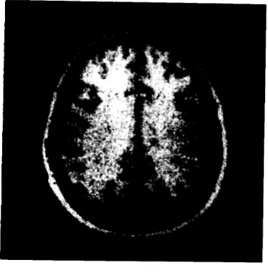
RESULTS
This method has been extensively tested on artificial and biomedical images (see Figs. 10-13) and performs very well. It correctly locates and traces all the borders shown in
Fig. 3 that were incorrectly traced by the
previous methods. It also correctly traced real images that were found to cause the other methods to fail. Furthermore the hole borders are better shaped, and more compact than those generated by the other methods when they did work. Thus this algorithm has proven superior to the previous methods of binary border following.
ACK"TS
The authors wish to express their gratitude to Mr. Ian Morris, of Queen Elizabeth I1 Medical Centre, for supplying the Magnetic Resonance Images used in this paper. The authors also wish to thank Mr Khanh Ly for
valuable discussions and providing
comparative algorithms.
This work was supported by an Australian Commonwealth Postgraduate Research Award and a research grant from The University of Western Australia. REFERENCES 1. 2. 3 . 4. 5 . 6. 7. 8.
Rosenfeld, A., and Kak, A.C., 1982,
Diqital Picture Processinq, 2nd ed.,
Vol. 2, Academic Press, New York.
Pavlidis, T., 1982, Alqorithms for
Graphics and Imacle Processinq, Springer- Verlag, Computer Science Press, MD.
Suzuki, S . , and Abe, K., 1985,
llTopological Structural Analysis of
Digital Binary Image by Border
Following", ComDut. Graphics Imaqe
Process., 30, 32-46.
Ly, K., and Attikiouzel, Y., 1987, "Contour Tracing of Biomedical Binary
Imagest1, Proc. Int. S V ~ D . Sianal
Process., Vol. 2, 735-738.
Kruse, B., 1980, "A Fast Stack
-
BasedAlgorithm for Region Extraction in
Binary and Nonbinary Images", Sisnal Processinq: Theories and Amlications, North-Holland Publishing Co., Amsterdam.
Danielsson, P. -E.
,
"An ImprovedSegmentation and Coding Algorithm for
Binary and Nonbinary Images", IBM J.
Res. Development, 26, 698-707.
Toriwaki, J.-I., and Yokoi, S , 1983,
I1Algorithms for Skeletonizing Three- Dimensional Digitized Binary Pictures",
Proc. SPIE, 435, 2-91.
Chen, B.-D., and Sir, P., 1987,
"Forward/Backward Contour Tracing with Feedback", IEEE Trans. Pat. Anal. Mach.
=,
pAMI-9, 3 , 438-446.0 0 0 0
k ff 0 0 0 0 0
0 0
:q
0 0d
0 0 0 0 0 0 0 0 0Which is better?
Figure 1. Connectivity paradox.
0 0 0 0 0
0 0 0
0 0 0 0 0 I m
length=%+4 length=12+1
0 0 0 0 0
0 0 0 0 0
length=4 length=4+4+4
0 0 0 0 0 0 0 0 0 0 0 0 0
0 0 0
0 0 0 0 0 0 0 0 0 0 0 0 0 0 0
Inner border Should be
not detected single object
0 0 0 0 0 0 0 0 0 0 0 0 0 0 0 0 Inner border masked
Figure 3. Incorrectly traced patterns.
0 0 0 0 0 m m m m m
0
:@:
0:E:
.
0 0 0 0 0
...
length=9 length=9
0 0 0 0 0
...
:%; :%;
...
0 0 0
0 0 0 0 0 m m m m m
length=4 length=4
Figure 4. Hole shape is improved (cf. Fig 2).
c frame
I i A
Figure 5. Topology of image.
Figure 6 . Chain code directions.
Pixel initially marked 0'
later changed to 0".
d' >d 0' d' <dn 0"
se&&able
Figure 7 . Local curvature.
no€- searchable
0 0 0 0 0 0 0
direction of
F&g:
0 0 0line scan
0 0
0 0 0 0 0 0 0
Figure 8 . Initial point may be re-entered.
Blocked
-
must OK OKskip direction
Figure 9. Examples of diagonal blocking.
t i j u r e 1:. Same image after thresholdlng Y-ijure 13. Degenerate b o r d e r s removed.