Bayesian Shrinkage estimators of the multivariate normal distribution

Bayesian Shrinkage estimators of the

multivariate normal distribution

Mutwiri Robert Mathenge

Department of mathematics and Actuarial science, Kirinyaga university P.O Box, 20-60215, Marimanti, Kenya

Abstract - This paper compares two shrinkage estimators of rates based on Bayesian methods. We estimate the mean θ of the multivariate normal distribution in 𝕽𝒑_{, when 𝝈}𝟐 _{is unknown using the chi-square random}

variable. The Modified Bayes estimator 𝜹𝑩∗and the Empirical Bayes estimator 𝜹𝑬𝑩∗ are considered and the

limits of their risk ratios of the maximum likelihood estimator when n andptend to infinity are obtained.

Keywords - Bayes estimator, Empirical Bayes estimator, James-Stein estimator , Multivariate Gaussian random variable, Modified Bayes estimator, Shrinkage estimator..

I.INTRODUCTION

Shrinkage estimation is a method to improve a raw estimator in some sense, by combining it with other information. Although the shrinkage estimator is biased, it is well known that it has minimum quadratic risk compared to natural estimators (mostly the maximum likelihood estimator) (Karamikabir, Afshari and Arashi, 2018). The shrinkage estimator, have evolved

over time since their introduction by Stein in 1956, James and Stein in 1961 and Stein in 1981. In these works one estimates the mean  by shrinking the empirical estimators of the mean, which are better in quadratic loss than the empirical mean estimator. More precisely, if

X represents an observation of a sample drawn from a multivariate normal distribution, the

aim is to estimate  by an estimator  relatively at the quadratic loss function 𝐿 𝛿, 𝜃 =∥ 𝛿 − 𝜃 ∥_𝑝2 _{where ∥. ∥}

𝑝the usual norm is inp and the associated risk function given by: R 𝛿, 𝜃 = 𝐸_𝜃 𝐿 𝛿, 𝜃 .

James and Stein (1961), introduced a class of estimators by improving 𝛿_𝜃 = 𝑋, when the dimension of the space of the observationsp 3, is denoted by :

𝛿_𝑗𝐽𝑆 = 1 −𝑝 − 2 𝑛 + 2

𝑆2

∥ 𝑋 ∥2 𝑋𝑗, 𝑗 = 1,2, … . , 𝑝

where 𝑆2~𝜎2𝜒_𝑛2 is the estimate of 𝜎2. Baranchik (1964), proposed the positive-part of James-Stein estimator dominating the James-Stein estimator when 𝑝 ≥ 3 ,

𝛿_𝑗𝐽𝑆 + = 𝑚𝑎𝑥 1 −𝑝−2_{𝑛+2∥𝑋∥}𝑆2₂ 𝑋_𝑗.

Casella and Hwang (1982), studied the case where 𝜎2 is known 𝜎2 = 1 and showed that if the limit of the ratio∥𝜃 ∥

2

𝑝 , when ptends to infinity is a constant 𝑐 > 0, then

lim𝑝→+∞ 𝑅 𝛿_{𝑅 𝑋,𝜃} 𝐽𝑆,𝜃 = lim𝑝→+∞𝑅 𝛿𝐽𝑆 +_,𝜃

𝑅 𝑋,𝜃 = 𝑐 1+𝑐.

Sun (1995), has considered the following model: 𝑦_𝑖𝑗 𝜎𝜃 2 ~𝑁 𝜃_𝑝, 𝜎2 ; 𝑖 =

1,2, … , 𝑛, 𝑗 = 1,2, … , 𝑚 where 𝐸(𝑦_𝑖𝑗) = 𝜃 for the group j and 𝑣𝑎𝑟(𝑦_𝑖𝑗) = 𝜎2 is unknown. The James-Stein estimator is written in 𝛿𝐽𝑆 = 𝛿₁𝐽𝑆, … , 𝛿_𝑚𝐽𝑆 ′, where

𝛿_𝑗𝐽𝑆 = 1 −(𝑚 −3)_(𝑁+2)𝑇𝑆2₂ 𝑦 _𝑗 − 𝑦 + 𝑦 , 𝑗 = 1,2, … , 𝑚, 𝑆2 = 𝑛_𝑖=1 𝑚_{𝑗 =1} 𝑦_𝑖𝑗 − 𝑦 _𝑗 2,

𝑇2 _{= 𝑛 𝑦} 𝑗 − 𝑦

2 𝑛

𝑖=0 , 𝑦 𝑖 = 𝑦𝑖𝑗 𝑛 𝑖=1

𝑛 and 𝑦 =

𝑦 𝑖 𝑚 𝑖=1

𝑚 , 𝑁 = 𝑛 − 1 𝑚.

𝛿_𝑗𝜓 = 1 − Ψ 𝑆2_{, 𝑇}2 _𝑦

𝑗 − 𝑦 + 𝑦 , 𝑗 = 1,2, … , 𝑚,

if lim_𝑝→+∞ 𝜃𝑗−𝜃

2 𝑛

𝑗 =1

𝑚 = 𝑞 exists, then lim𝑚→+∞

𝑅(𝛿𝜓,𝜃) 𝑅(𝑋,𝜃) ≥

𝑞

𝑞+𝜎2_𝑛 and

lim_𝑚→+∞𝑅(𝛿_{𝑅(𝑋,𝜃 )}𝐽𝑆,𝜃)= lim_𝑚→+∞𝑅(𝛿_{𝑅(𝑋,𝜃)}𝐽𝑆 +,𝜃 )≥ 𝑞

𝑞+𝜎2_𝑛.

where 𝑞

𝑞 +𝜎2_𝑛 constitutes a lower bound for the ratio lim𝑚→+∞

𝑅(𝛿𝜓_{,𝜃 )}

𝑅(𝛿0,𝜃) and is equal to

lim𝑚→+∞𝑅(𝛿 𝐽𝑆_{,𝜃 )}

𝑅(𝛿0,𝜃 ).

Sun (1995), also showed that this bound is attained for a class of estimators defined by:

𝛿_𝑗 = 1 − Ψ 𝑆2_{, 𝑇}2 _𝑦

𝑗 − 𝑦 + 𝑦 , 𝑗 = 1,2, … , 𝑚 where Ψ satisfies certain conditions.

This bound is also attained for any estimator dominating the James-Stein estimator, in particular the positive-part.

Further, we note that if n tends to infinity then the ratio 𝑞

𝑞+𝜎2_𝑛 tends to 1, and thus the risk

of the James-Stein estimator is that of 𝛿₀ (when n andmtend to infinity).

Hamdaoui and Benmansour (2015), considered the following class of shrinkage estimators 𝛿_𝜓 = 𝛿_𝐽𝑆 + 𝜄𝜓 𝑆2, ∥ 𝑋2 ∥ 𝑋, which is introduced in Benmansour and Mourid (2007). The authors showed that if lim_𝑚→+∞∥𝜃 ∥

2

𝑝 = 𝑐(> 0) then the risk ratios 𝑅(𝛿𝜓,𝜃)

𝑅(𝑋,𝜃) , 𝑅(𝛿𝐽𝑆_,𝜃)

𝑅(𝑋,𝜃 ) and

𝑅(𝛿𝐽𝑆 +_{,𝜃 )}

𝑅(𝑋,𝜃) attain the lower bound 𝐵𝑚 = 𝑐

1+𝑐when n and ptend to infinity provided

that lim

𝑚 →+∞ ∥𝜃∥2

𝑝 . Hamdaoui and Mezouar (2017), considered the general class of

shrinkage estimators 𝛿_𝜓 = 1 − 𝜓 𝑆2, ∥ 𝑋2 ∥ 𝑆

2

∥𝑋2_∥ X. The authors showed the same

results given by Hamdaoui and Benmansour (2015), under different conditions from the one

given by Hamdaoui and Benmansour (2015). When the dimensionpis finite, Brandwein

and Strawderman (2012) considered the following model (𝑋, 𝑈) ∼ 𝑓 ∥ 𝑋 − 𝜃 ∥2 +∥ 𝑈 ∥2 , where dim 𝑋 = dim 𝜃 = 𝑝 and dim 𝑈 = 𝑘. The classical example of this model is, of

course, the normal model of density 1

2𝜋𝜎 𝑝+𝑘

𝑒−|𝑥−𝜃 |22𝜎2 _{. They showed that the estimator}

𝛿 = 𝑋 + 𝑈 _𝑘+22 𝑔(𝑋) dominatesX , so that is Minimax, provided the function g satisfies certain conditions.

Maruyama (2014) has also studied the minimaxity of shrinkage estimator when the dimension of parameter’s space is moderate. Then he considered the following model

𝑍 ∼ 𝑁(𝜃, 𝐼_𝑑) and the so called 𝜋 -norm given by: ∥ 𝑍 ∥_𝑝= 𝑛_𝑖=0|𝑧_𝑖|𝑝

1

𝑝, 𝑝 > 0_{. He}

studied the minimaxity of shrinkage estimators defined as follows: 𝜃 _𝜙 = 𝜃 _1𝜙, … , 𝜃 _𝑑𝜙 with: 𝜃 _𝑖𝜙 = 1 − 𝜙 ∥ 𝑍 ∥_𝑝 /𝜙 ∥ 𝑍 ∥_𝑝2−𝛼 |𝑍_𝑖|𝛼 where 0 ≤ 𝛼 ≤ (𝑑 − 2)/(𝑑 − 1) and

𝑝 > 0. Note that the risk functions of these estimators are calculated relatively to the usual quadratic loss function defined at above.

In this work we adopt the model 𝑋~𝑁𝑝 𝜃, 𝜎2𝐼𝑝 such that the parameter 𝜎2is

the hyperparameter 2is known or unknown. The aim is estimating the mean 𝜃 by a the Modified Bayes estimator 𝛿_𝐵∗ when the hyperparameter 𝜏2 is known and by an Empirical Bayes estimator 𝛿_𝐸𝐵∗ when the hyperparameter 𝜏2 is unknown. Note that 𝑅(𝑋; 𝜃) = 𝑝𝜎2, is the risk of the Maximum likelihood estimator.

In section 1, we recall some technical’s Lemmas that we use them for later and we also recall some results linked with Bayes estimators of the mean of a multidimensional normal distribution.

In Section 2, we give the main results of this paper. First, we take the prior low of:

𝜃~𝑁_𝑝 𝜈, 𝜏2_𝐼

𝑝 where the hyperparameters 𝜈, 𝜏2 are known and we construct a Modified

Bayes estimator 𝛿_𝐵∗ of the mean 𝜃, then we study the minimaxity of this estimator when n

andpare fixed. In the second part of this section we study the behaviour of the risk ratio of this estimator to the Maximum likelihood estimator X when n and ptend to infinity.

In the section 3, we take the prior distribution of 𝜃: 𝜃~𝑁_𝑝 𝜈, 𝜏2𝐼_𝑝 where the

hyperparameter 𝜈 is known and the hyperparameter 𝜏2 is unknown and we construct an Empirical Bayes estimators of the mean 𝜃, then we will follow the same steps as we have given in section two. In the end we illustrate graphically the risk ratios of the Modified Bayes estimator 𝛿_𝐵∗to the Maximum likelihood estimator X for divers values of n.

II.PRELIMINARIES

We recall that if X is a multivariate Gaussian random 𝑁𝑝 𝜃, 𝜎2𝐼𝑝 in p then ∥𝑋∥ 2

𝜎2 ~𝜒𝑞2 𝜆

where 𝜒_𝑞2 𝜆 denotes the non-central chi-square distribution with p degrees of freedom and non-centrality parameter 𝜆 =∥𝜃∥

2

2𝜎2. We recall the following Lemmas that we will use often

in our proofs.

Lemma 2.1 (Fourdrinier et. al., 2007)

Let 𝑋~𝑁𝑝 𝜃, 𝜎2𝐼𝑝 , 𝜃 ∈ ℜ𝑝. Then, for 𝑝 ≥ 3, we have 𝐸 _∥𝑋12_∥ = 1 𝜎2𝐸

1

𝑝−2+2𝑘 , where

𝑋~𝑃 ∥𝜃 ∥_2𝜎22 , being the Poisson’s distribution of the parameter∥𝜃∥_2𝜎22.

Lemma 2.2 (Stein 1981)

LetYbe a 𝑁(0,1) real random variable and let 𝑔: ℜ → ℜ be an indefinite integral of the

Lesbegue measurable function '

g , essentially the derivative of g. Suppose also that

𝐸 𝑔′(𝑌) < ∞. Then 𝐸 𝑌𝑔 𝑌 = 𝐸(𝑔′ 𝑌 ).

Lemma 2.3 (Casella and Hwang, 1982)

For any real function h such that 𝐸 𝑕 𝜒_𝑞2 𝜆 𝜒_𝑞2 𝜆 exists, we have

𝐸 𝑕 𝜒𝑞2 𝜆 𝜒𝑞2 𝜆 = 𝑞𝐸 𝑕 𝜒𝑞+22 𝜆 + 2𝜆𝐸 𝑕 𝜒𝑞+22 𝜆

Lemma 2.4 (Benmansour and Hamdaoui, 2011)

Let f is a real function. If for 𝑝 ≥ 3, 𝐸_𝜒𝑞2 _𝜆 𝑓(𝑈) exists, then

a) If f is monotone non-increasing we have

𝐸_{𝜒𝑝 +2}2 _𝜆 𝑓(𝑈) ≤ 𝐸_𝜒

b) If f is monotone non-decreasing we have

𝐸_{𝜒𝑝 +2}2 _𝜆 𝑓(𝑈) ≥ 𝐸_𝜒𝑝2 _𝜆 𝑓(𝑈) . (2.2)

We also recall in what follows a few results of Bayes estimator.

Let 𝑋/𝜃~𝑁_𝑝 𝜃, 𝜎2𝐼_𝑝 and 𝜃~𝑁_𝑝 𝜈, 𝜏2𝐼_𝑝 where 𝜎2 known, and hyperparameters is

𝜈, 𝜏2 _{are known. Then from Lindley (1972), we have}









p B X BI

N

X ~









2

𝜏2_+𝜎2, then the Bayes estimator of 𝜃 is

𝛿_𝐵 𝑋 = 𝐸 _𝑋𝜃 = 𝜐 + 𝐵(𝑋 − 𝜐) thus

𝛿𝐵 𝑋 = 1 − 𝜏 2

𝜏2_+𝜎2 𝑋 − 𝜐 +. (2.3)

We deduce that

i) 𝑅 𝛿_𝐵 𝑋 ; 𝜃 = 1 − 𝐵 2∥ 𝜃 − 𝜐 ∥2+ 𝐵2𝑝𝜎2

and

ii) 𝑅 𝛿𝐵 𝑋 ; 𝜈,𝜏 2_,𝜎2

𝑅(𝑋) =

𝜏2 𝜏2_+𝜎2

III.RESULTSANDDISCUSSION

In this section we are interested in studying the minimaxity, bounds and limits of risk ratios of the Modified Bayes and the Empirical Bayes estimators, to the Maximum likelihood estimator X. In the next, we give the following Lemma.

Lemma 3.1

For any c > 0, we have:

1

𝑛+2+𝑐 ≤ 𝐸𝜒𝑛 +22 1 𝑢+𝑐 ≤

1

𝑛+𝑐, (3.1)

1

𝑛+4+𝑐 2 ≤ 𝐸𝜒𝑛 +42 1 𝑢+𝑐 2 ≤

1

𝑛+𝑐 2 (3.2)

Proof

From Jensen’s inequality we have .

𝐸_{𝜒𝑛 +2}2 1 𝑢+𝑐 ≥

1 𝑛+2+𝑐.

On the other hand, from lemma 2.3, we have

1 = 𝐸_𝜒𝑛2 𝑢

𝑢 + 𝑐 + 𝑐𝐸𝜒𝑛 +22

1 𝑢 + 𝑐 = 𝑛𝐸_{𝜒𝑛 +2}2 1

𝑢 + 𝑐 + 𝑐𝐸𝜒𝑛2

1 𝑢 + 𝑐

Then

𝐸_{𝜒𝑛 +2}2 1 𝑢+𝑐 =

1

𝑛 1 − 𝑐𝐸𝜒𝑛2 1 𝑢+𝑐 ≤

1

𝑛+𝑐 .

The last inequality follows from Jensen’s inequality. The proof of the formula (3.2) is as follows: from Jensen’s inequality we have

𝐸_{𝜒𝑛 +4}2 1 𝑢+𝑐 2 ≤

1

𝑛+4+𝑐 2 .

𝐸_{𝜒𝑛 +2}2 1

𝑢 + 𝑐 = 𝐸𝜒𝑛 +22

𝑢

𝑢 + 𝑐 2 + 𝑐𝐸𝜒𝑛 +22

1 𝑢 + 𝑐 2

= (𝑛 + 2)𝐸_{𝜒𝑛 +4}2 1

𝑢+𝑐 2 + 𝑐𝐸𝜒𝑛 +22 1

𝑢+𝑐 2 (3.3)

≥ 𝑛 + 2 𝐸_{𝜒𝑛 +4}2 1

𝑢+𝑐 2 + 𝑐𝐸𝜒𝑛 +22 1

𝑢+𝑐 2 (3.4)

≥ (𝑛 + 2 + 𝐶)𝐸_{𝜒𝑛 +4}2 1

𝑢 + 𝑐 2

The equality (3.3) follows from Lemma 2.3 and the inequality (3.4) follows to the formula (2.1) of Lemma 2.4. Hence

𝐸_{𝜒𝑛 +2}2 1

𝑢 + 𝑐 2 ≤

1

𝑛 + 2 + 𝑐𝐸𝜒𝑛 +22

1 𝑢 + 𝑐

Using the formula (3.1), we obtain

𝐸_{𝜒𝑛 +2}2 1 𝑢+𝑐 2 ≤

1 𝑛+2+𝑐

1 𝑛+𝑐 ≤

1 𝑛+𝑐 2.

Modified Bayes Estimator

Let 𝑋/𝜃~𝑁_𝑝 𝜃, 𝜎2𝐼_𝑝 and 𝜃~𝑁_𝑝 𝜈, 𝜏2𝐼_𝑝 where 𝜎2 is unknown, and the hyperparameters 𝜈, 𝜏2 are known. We note that 𝑆

2

𝑆2_+𝑛𝜏2 is an asymptotically unbiased

estimator of ratio 𝜎2

𝜎2_+𝜏2. Endeed

𝐸 𝑆2

𝑆2_{+ 𝑛𝜏}2 = 𝐸

𝑆2

𝜎2

𝑆2

𝜎2+ 𝑛 𝜏 2

𝜎2

= 𝑛𝐸_𝜒

𝑛 +22

𝑆2

𝑢 + 𝑛 𝜏_𝜎2₂

The last equality comes from Lemma 2.3. From the previous equality and the formula (3.1) of Lemma 3.1, we obtain

𝑛

𝑛 1+_𝜎2𝜏2 +2 ≤ 𝐸 𝑆2 𝑆2_+𝑛𝜏2 ≤

𝑛 𝑛 1+_𝜎2𝜏2 ,

It is clear that both the upper and the lower bound converge to 𝜎2

𝜎2_+𝜏2 when 𝑛 → ∞. Thus

lim_𝑛→∞ 𝐸 _{𝑆2+𝑛𝜏}𝑆2 ₂ =_𝜎2𝜎_+𝜏2₂.

If we replace in formula (2.3) the ratio 𝜎

2

𝜎2_+𝜏2 by its estimator 𝑆2

𝑆2_+𝑛𝜏2, we obtain the

Modified Bayes estimator expressed as

𝛿_𝐵∗ _{= 1 −} 𝑆2

𝑆2_+𝑛𝜏2 𝑋 − 𝜐 + 𝜐 (3.5)

Proposition 3.2

Let the Modified Bayes estimator 𝛿_𝐵∗ given in (3.5), then i) The risk function of the estimator 𝛿_𝐵∗ is

𝑅 𝛿𝐵∗; 𝜈, 𝜏2, 𝜎2 = 𝑝𝜎2+ 𝑝𝜎2 𝑛 𝑛 + 2 1 + 𝜏2 𝜎2 𝐸𝜒_{𝑛 +4}2

1

𝑢 + 𝑛 𝜏_𝜎22

2 − 2𝑛𝐸𝜒_{𝑛 +2}2 1

𝑢 + 𝑛 𝜏_𝜎22

ii)1 +𝑛(𝑛+2) 1+

𝜏2 𝜎2

𝑛 1+𝜏2 𝜎2 +4

2− 2 1+_𝜎2𝜏2 ≤

𝑅 𝛿𝐵∗;𝜈 ,𝜏2,𝜎2

𝑅(𝑋) ≤ 1 + 𝑛+2 𝑛 1+𝜏2_𝜎2 −

2𝑛 𝑛 1+_𝜎2𝜏2 +2.

Proof

 

















n S

S E

R _B

From the independence to two variables X andS2, we have

𝑅 𝛿𝐵∗; 𝜃 = 𝐸𝜃 ∥ 𝑋 − 𝜃 ∥2 + 𝐸𝜃 𝑆2 𝑆2_{+ 𝑛𝜏}2

2

𝐸𝜃 ∥ 𝑋 − 𝜐 ∥2 − 2𝜎2𝐸𝜃 𝑆2

𝑆2_{+ 𝑛𝜏}2 𝐸𝜃 𝑋 − 𝜃

𝜎 , 𝑋 − 𝜈

𝜎

= 𝑝𝜎2+𝐸_{𝜒𝑛 +2}2 𝑢

𝑢+𝑛𝜏2

𝜎 2

2

𝑝𝜎2_{+∥ 𝜃 − 𝜐 ∥}2_{− 2𝑛𝑝𝜎}2_𝐸 𝜒_𝑛2 𝑢

𝑢+𝑛𝜏2

𝜎 2

(3.6)

= 𝑝𝜎2+𝑛(𝑛 + 2)𝐸_{𝜒𝑛 +4}2 1

𝑢+𝑛𝜏2

𝜎 2

2 𝑝𝜎2+∥ 𝑋 − 𝜃 ∥2− 2𝑛𝑝𝜎2 𝐸𝜒_{𝑛 +2}2 1 𝑢+𝑛𝜏2

𝜎 2 .

The equality (3.6) according to the Lemma 2.2 and the last equality follow from Lemma 2.3. Thus

𝑅 𝛿_𝐵∗_{; 𝜈, 𝜏}2_{, 𝜎}2 _{= 𝐸}

𝛿_𝐵∗;𝜈,𝜏2_,𝜎2 𝑅(𝛿_𝐵∗; 𝜃)

= 𝑝𝜎2_{+𝑛(𝑛 + 2)𝐸} 𝜒𝑛 +42

1

𝑢 + 𝑛 𝜏_𝜎2₂ 2

𝑝𝜎2_{+ 𝐸}

𝜒_𝜐,𝜏22 |𝑋 − 𝜃|2 − 2𝑛𝑝𝜎2 𝐸𝜒_{𝑛 +2}2 1

𝑢 + 𝑛 𝜏_𝜎2₂

= 𝑝𝜎2_{+ 𝑝𝜎}2 _{𝑛 𝑛 + 2 1 +}𝜏2

𝜎2 𝐸𝜒𝑛 +42

1

𝑢 + 𝑛 𝜏_𝜎22

2 — 2𝑛𝐸𝜒_{𝑛 +2}2 1

𝑢 + 𝑛 𝜏_𝜎2₂ From i) we have

𝑅 𝛿𝐵∗; 𝜈, 𝜏2, 𝜎2

𝑅(𝑋) = 1 + 𝑛 𝑛 + 2 1 + 𝜏2

𝜎2 𝐸𝜒_{𝑛 +2}2 − 2𝑛𝐸𝜒_{𝑛 +2}2 1 𝑢 + 𝑛 𝜏_𝜎2₂

Using formulas (3.1) and (3.2) of Lemma 3.1, we obtain

𝑅 𝛿𝐵∗; 𝜈, 𝜏2, 𝜎2

𝑅(𝑋) ≤ 1 + 𝑛 𝑛 + 2 1 + 𝜏2 𝜎2

1

𝑛 + 𝑛 𝜏_𝜎2₂ 2

− 2𝑛

𝑛 + 2 + 𝑛 𝜏_𝜎22

≤ 1 + 𝑛+2 𝑛 1+𝜏2

𝜎 2

− 2𝑛

𝑛 1+𝜏2

𝜎 2 +2 and

𝑅 𝛿𝐵∗; 𝜈, 𝜏2, 𝜎2

𝑅(𝑋) ≥ 1 + 𝑛 𝑛 + 2 1 + 𝜏2 𝜎2

1

𝑛 + 4 + 𝑛 𝜏_𝜎2₂ 2

− 2𝑛

𝑛 + 2 + 𝑛 𝜏_𝜎22

≥ 1 + 𝑛 𝑛+21+ 𝜏2 𝜎 2

𝑛 1+𝜏2

𝜎 2 +4 2−

2

1+_{𝜎 2}𝜏2

Theorem 3.3

a) If 𝑝 ≥ 3 and 𝑛 ≥ 5 the estimator 𝛿_𝐵∗ given in (3.5) is minimax, b) lim_{𝑛,𝑝→∞}𝑅 𝛿𝐵

∗_;𝜈,𝜏2_,𝜎2

𝑅(𝑋) = 𝜏2 𝜏2+𝜎2.

Proof

a) From the previous Proposition, we have

𝑅 𝛿_𝐵∗_{; 𝜈, 𝜏}2_{, 𝜎}2 _{≤ 𝑝𝜎}2 _{+ 𝑝𝜎}2 𝑛(𝑛 + 2) 1 + 𝜏2 𝜎2

𝑛 + 𝑛_𝜎𝜏22

2 −

2𝑛 𝑛 + 2 + 𝑛_𝜎𝜏22

The study of the variation of the real function 𝑕 𝑥 = 𝑥+2

𝑥 1+𝜏2

𝜎2

− 2𝑛

𝑥 1+𝜏2

𝜎2 +2

, shows that

(𝑛+2) 𝑛 1+_𝜎2𝜏2 −

2𝑛

𝑛 1+_𝜎2𝜏2 +2≤ 0 for any 𝑛 ≥ 5,

Then 𝑅 𝛿_𝐵∗; 𝜈, 𝜏2, 𝜎2 ≤ 𝑅(𝑋) ≤ 𝑝𝜎2 for any 𝑛 ≥ 5. Thus 𝛿_𝐵∗ is minimax for any 𝑛 ≥ 5.

b) Immediately from ii) of the Proposition 3.2.

Empirical Bayes estimator

Let 𝑋/𝜃~𝑁_𝑝 𝜃, 𝜎2𝐼_𝑝 and 𝜃~𝑁_𝑝 𝜈, 𝜏2𝐼_𝑝 where 𝜎2 is unknown and the hyperparameter 𝜈 is known and the hyperparameter 𝜏2is unknown. We note that

𝑝−2 𝑛+2

𝑆2

𝑋−𝜐 2 (where𝑆2~𝜎2𝜒𝑛2 ) is an asymptotically unbiased estimator of ratio 𝜎2

𝜎2_+𝜏2. Endeed:

from the independence to two variables 𝑆2and 𝑋 2, we have

𝐸 𝑝 − 2 𝑛 + 2

𝑆2

𝑋 − 𝜐 2 =

𝑝 − 2 𝑛 + 2

𝜎2

𝜎2_{+ 𝜏}2𝐸

𝑆2

𝜎2 𝐸

1 𝑋 − 𝜐 2

𝜎2 _{+ 𝜏}2

As the marginal distribution of X is 𝑋~𝑁_𝑝 𝜐, (𝜎2+ 𝜏2)𝐼_𝑝 , then 𝑋−𝜐

2

𝜎2_+𝜏2 ~𝜒𝑝2.

Using the Lemma 2.1, we obtain 𝐸 _{𝑋 −𝜐 2}1

𝜎2+𝜏2

= 𝐸 _𝜒1

𝑝2 = 1

𝑝−2, thus

𝐸 𝑝−2_{𝑛+2 𝑋−𝜐} 𝑆2 ₂ =_𝑛+2𝑛 _𝜎2𝜎_+𝜏2₂

𝑛→∞

_𝜎2𝜎_+𝜏2 ₂.

If we replace in formula (2.3) the ratio 𝜎2

𝜎2_+𝜏2by its estimator 𝑝−2 𝑛+2

𝑆2

𝑋−𝜐 2, we obtain the

Empirical Bayes estimator expressed as

𝛿_𝐸𝐵∗ _{= 1 −}𝑝−2 𝑛+2

𝑆2

𝑋−𝜐 2 𝑋 − 𝜐 + 𝜐 (3.7)

Proposition 3.4

The risk function of the Empirical Bayes estimator 𝛿_𝐸𝐵∗ given in (3.7) is

𝑅 𝛿_𝐸𝐵∗ _{; 𝜈, 𝜏}2_{, 𝜎}2 _{= 𝑝𝜎}2 _{1 −}𝑝−2 𝑝

𝑛 𝑛+2

𝜎2 𝜎2_+𝜏2 .

Proof

𝑅 𝛿𝐸𝐵∗ ; 𝜈, 𝜏2, 𝜎2 = 𝐸 1 − 𝑝 − 2 𝑛 + 2

𝑆2

𝑋 − 𝜐 2 𝑋 − 𝜐 + 𝜐 − 𝜃 2

= 𝐸 𝑋 − 𝜃 2 ₊ 𝑝 − 2 𝑛 + 2

2 _𝜎4

𝜎2_{+ 𝜏}2𝐸 𝑆2 𝜎2 𝐸

1 𝑋 − 𝜐 2

𝜎2_{+ 𝜏}2

−𝑛(𝑝 − 2) 𝑛 + 2 𝜎2𝐸

𝑆2 𝜎2 𝐸

𝑋 − 𝜃 𝜎 ,

1 𝑋 − 𝜐 2

𝜎2

𝑋 − 𝜐 𝜎

Using Lemma 2.2, we obtain

𝐸 𝑋 − 𝜃 𝜎 ,

1 𝑋 − 𝜐 2

𝜎2

𝑋 − 𝜐

𝜎 = 𝐸 𝑋 − 𝜃𝜎 1 𝑋 − 𝜐 2

𝜎2

𝑋 − 𝜐 𝜎 𝑝

𝑖=1

= 𝐸 𝜕 𝜕𝑋𝑖

1 𝑋 − 𝜐 2

𝜎2

𝑋 − 𝜐 𝜎 𝑝

𝑖=1

= 𝑝 − 2 𝐸 _𝑋−𝜐1 2 𝜎2

= (𝑝 − 2)_𝜎2𝜎_+𝜏2 ₂𝐸 _𝑋−𝜐1 2 𝜎2

= 𝑝 − 2 𝜎

2

𝜎2_+𝜏2𝐸 1 𝜒𝑝2 =

𝜎2

Because 𝑋−𝜐 _𝜎2 2~𝜒_𝑝2 _{and 𝐸} 1 𝜒𝑝2 =

1

𝑝−2. Thus, 𝑅 𝛿𝐸𝐵

∗ _{; 𝜈, 𝜏}2_{, 𝜎}2 _{= 𝑝𝜎}2 _{1 −}𝑝−2 𝑝

𝑛 𝑛+2

𝜎2 𝜎2_+𝜏2 .

Theorem 3.5

Let the Empirical Bayes estimator 𝛿_𝐸𝐵∗ given in (3.7), then a) If 𝑝 ≥ 3, the estimator 𝛿_𝐸𝐵∗ is minimax,

b) lim_{𝑛,𝑝→∞}𝑅 𝛿𝐸𝐵

∗ _{;𝜈 ,𝜏}2_,𝜎2

𝑅(𝑋) =

𝜏2 𝜏2+𝜎2

Proof

Immediately from the Proposition 3.4.

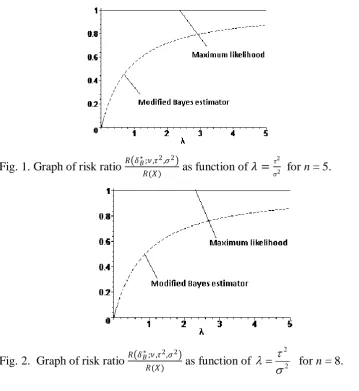
IV.SIMULATIONRESULTS

We illustrate graphically the performance of the risk ratios of the Bayes estimator 𝛿𝐵∗ to the Maximum likelihood estimatorX expressed as𝑅 𝛿𝐵

∗_;𝜈,𝜏2_,𝜎2

𝑅(𝑋) as a function of 𝜆 = 𝜏2

𝜎2 for various values of n.

Fig. 1. Graph of risk ratio 𝑅 𝛿𝐵

∗_;𝜈,𝜏2_,𝜎2

𝑅(𝑋) as function of 𝜆 =

𝜏2

𝜎2 for n = 5.

Fig. 2. Graph of risk ratio 𝑅 𝛿𝐵

∗_{;𝜈 ,𝜏}2_,𝜎2

𝑅(𝑋) as function of 2

2  

  for n = 8.

V.CONCLUSIONS

function. We take the same model 𝑋~𝑁_𝑝 𝜃, 𝜎2𝐼_𝑝 with the unknown 𝜎2 estimated by the statistic 𝑆2~𝜎2𝜒_𝑛2 independent of X, given the prior distribution 𝜃~𝑁_𝑝 𝜈, 𝜏2𝐼_𝑝 where the hyperparameter is known and the hyperparameter 𝜏2 is known or unknown, then we constructed the Modified Bayes estimator 𝛿_𝐵∗ when the hyperparameter 𝜏2is known and the Empirical Bayes estimator 𝛿_𝐸𝐵∗ when the hyperparameter 𝜏2 is unknown and showed that the estimators 𝛿_𝐵∗ and 𝛿_𝐸𝐵∗ are Minimax when n and p are finite. When n and p tend simultaneously to infinity without assuming any order relation or functional relation

between n and p, we showed that the risk ratios 𝑅 𝛿𝐵

∗_{;𝜈 ,𝜏}2_,𝜎2

𝑅(𝑋) and

𝑅 𝛿𝐸𝐵∗ ;𝜈 ,𝜏2,𝜎2

𝑅(𝑋) tend to the

same value 𝜏

2

𝜏2_+𝜎2which is less than 1. An idea would be to see whether one can obtain

similar results of the asymptotic behaviour of risk ratios in the general case of the symmetrical spherical models, for general classes of shrinkage estimators.

REFERENCES

[1] Baranchik, A.J., 1964. Multiple regression and estimation of the mean of a multivariate normal distribution. Stanford Univ. Technical Report.

[2] Benmansour, D. and Hamdaoui, A., 2011. Limit of the Ratio of Risks of James-Stein Estimators with Unknown Variance. Far East J. Theorical Stat., 36: 31-53. https://www.statindex.org/articles/257944.

[3] Benmansour, D. and Mourid, T., 2007. Etude d’une classe d’estimateurs avec rétrécisseur de la moyenne d’une loi gaussienne. Annales de l.ISUP, Fascicule, 51: 1-2.

[4] Brandwein A.C. and Strawderman, W.E. Stein Estimation for Spheri-cally Symmetric Distributions : Recent Developments, Statistical Science,27(1), 2012, 11-23.

[5] Casella, G. and Hwang, J.T., 1982. Limit expressions for the risk of James-Stein estimators. Canadian J. Stat., 10: 305-309. DOI: 10.2307/3556196

[6] Fourdrinier, D., Ouassou I. and Strawderman, W.E. 2008. Estimation of a mean vector under quartic loss. J. Stat. Plann. Inference, 138: 3841-3857. DOI: 10.1016/j.jspi.2008.02.009

[7] Hamdaoui, A. and Benmansour, D., 2015. Asymptotic properties of risks ratios of shrinkage estimators. Hacettepe J. Math. Stat., 44: 1181-1195. DOI: 10.15672/HJMS.2014377624.

[8] Karamikabir, H., Afshari, M., & Arashi, M., 2018. Shrinkage estimation of non-negative mean vector with unknown covariance under balance loss. Journal of inequalities and applications, 2018(1), 331. doi:10.1186/s13660-018-1919-0

[9] Hamdaoui, A. and Mezouar, N., 2017. Risks Ratios of shrinkage estimators for the multivariate normal mean. Journal of Mathematics and Statistics, Science Publication., 13(2): 77-87. DOI: 10.3844/jmssp.2017.77.87.

[10] James, W. and Stein, C., 1961. Estimation of quadratique loss.

[11] Proceedings of the 4th Berkeley Symp., Math. Statist. Prob., (MSP’ 61), Univ of California Press, Berkeley, pp: 361 -379. [12] Lindley, D. V. And Smith A. F. M. Bayes estimates for the linear model (with discussion). J. Roy. Statist. Soc. B 34, 1-41,

(1972).

[13] Maruyama, Y., 2014. lp-norm based James-Stein estimation with minimaxity and sparsity. Statistics Theory (math.ST) arXiv. [14] Stein, C., 1956. Inadmissibilty of the usual estimator for the mean of a multivariate normal distribution. Proceedings of the 3th

Berkeley Symp., Math. Statist. Prob., (MSP’ 56), Univ. of California Press, Berkeley, pp: 197-206.

[15] Stein, C., 1981. Estimation of the mean of a multivariate normal distribution. Ann. Stat., 9: 1135-1151. DOI: 10.1214/aos/1176345632A.C.