∀+1(0.2//03456/6/2
7) ∃#88 ∋ ∗8058
Special Session
Optimisation Methods – Novel Aspects
Keynote: Algorithms Applied to Global Optimisation – Visual Evaluation Dr Kalin Penev, Southampton Solent University
Algorithms Applied to Global Optimisation – Visual Evaluation
Kalin Penev
Southampton Solent University, Southampton, UK
Abstract: Evaluation and assessment of various search and optimisation algorithms is subject of large research efforts. Particular interest of this study is global optimisation and presented approach is based on observation and visual evaluation of Real-Coded Genetic Algorithm, Particle Swarm Optimisation, Differential Evolution and Free Search, which are briefly described and used for experiments. 3D graphical views, generated by visualisation tool VOTASA, illustrate essential aspects of global search process such as divergence, convergence, dependence on initialisation and utilisation of accidental events. Discussion on potential benefits of visual analysis, supported with numerical results, which could be used for comparative assessment of other methods and directions for further research conclude presented study.
Keywords: Search Process Visualisation, Real-Coded Genetic Algorithm, Particle Swarm Optimisation, Differential Evolution, Free Search, Numerical Optimization.
1. Introduction
Global optimization refers to finding optimal solution of a given non-convex objective function [6][14]. Real world tasks are often global and need reliable methods to cope with. For this purpose various search methods such as Genetic Algorithm [7], Particle Swarm Optimization (PSO) [2][3], Differential Evolution [13] and Free Search (FS) [9][10] can be used. However majority of search and optimization methods face difficulties when dealing with global optimization problems. The main reasons of their failure are: trap in local sub-optimal solution, inability to escape from trapping, inability to abstract appropriate knowledge or use it effectively (if available).
Observation of optimisation process and visual analysis significantly help to identify dependence on initialisation of some methods, abilities to diverge across the whole search space, abilities to converge to optimal solution, abilities to use accidental events and to abstract from them knowledge, which could facilitate search process. This study uses for experiments Real-Coded Genetic Algorithm, Particle Swam Optimisation, Differential Evolution and Free Search.
1.1. Genetic Algorithm
1.2. Particle Swarm Optimisation
PSO can be classified as a population-based, evolutionary computational paradigm [2]. It has been compared to Genetic Algorithms [1][3] for efficiently finding optimal or near-optimal solutions in large search spaces. PSO is different from other evolutionary computational methods. It attempts to model a social behaviour of a group of individuals [2][12]. In PSO each particle is defined as a potential solution to a problem in multi-dimensional space. One of the advantages of PSO is flexible tuning of few parameters. One version, with slight variations, works well in a wide variety of applications. A variable called inertia factor influences PSO positively. Large inertia factor facilitates global exploration and searching new areas, while small inertia factor tends to facilitate local exploration and fine-tunes the current search area [5].
1.3. Differential Evolution
Differential Evolution can be described as real-value method for optimising non-linear and non-differentiable functions within continuous space [11][13]. It starts with stochastic selection of an initial set of solutions called design vectors. The value of an objective function, which corresponds to each individual of the population, is a measure of that individual’s fitness as an optimum. Then, guided by the principle of survival of the fittest, the initial population of vectors is transformed, generation-by-generation, into a solution vector. DE selects for manipulation target, donor and differential vectors. Therefore the minimal number of vectors in one population has to be more than four. For modification strategies, which use four differential vectors the minimal population size is seven. The current target and corresponding new trial vector (individual) in each generation are subject of competitions to determine the composition of the next generation. The new trail vector is generated in several steps as follows: (1) selection of a randomly chosen donor vector from the population different from the current target vector; (2) selection of other (two or four) randomly chosen vectors (so called differential vectors), different from the donor, different from the current target vector and different from each other; (3) calculation of a difference between differential vectors and scaling it by multiplication with a constant called differential factor; (4) adding the difference to the donor vector, which produces a new vector; (5) crossover between the current target vector and the new vector so that the trial vector inherits parameters from both of them. If the trial vector is better than the current target vector, then the trial vector replaces the target vector in the next generation. In all, three factors control evolution under DE: the population size; the scaling weight (differential factor) applied to the random vectors differential.
1.4. Free Search
Free Search is real-value adaptive heuristic method. The search process is organised in exploration walks, which differs from classical iterations [9][10]. It starts with initialisation. The algorithm requires definition of the search space boundaries [Xmini and Xmaxi],
population size m, limit for the number of explorations G, limit for the number of steps for exploration T, minimal and maximal values for the frame of a neighbourhood space [Rmin,
FS requires definition of an initialisation strategy. Acceptable initialisation strategies are: - random values: x0ji= Xmini + (Xmaxi– Xmini)*randomji(0,1), (1)
- certain values: x0ji= aji, aji [Xmini, Xmaxi], (2)
- one location: x0ji= ci, ci [Xmini, Xmaxi], (3)
where random(0,1) is a random value between 0 and 1, aji and ci are constants.
The ability to operate with all these strategies also supports good performance across a variety of problems without constant re-tuning of internal operator parameters. For multi-start optimisation FS allows variation of the initialisation strategies. Upon initialisation each individual takes an exploratory walk. It generates coordinates of a new location xtji as:
xtji = x0ji- xtji+ 2*xtji*randomtji(0,1). (4)
Modification strategy used in the algorithm is:
xtji = Rji * (Xmaxi – Xmini) * randomtji(0,1), (5)
where i = 1 for a one-dimensional step (l indicates one dimension); i = 1,..,n for a multi-dimensional step. t is the current step t = 1,..,T. T is the step limit per walk. Rji indicates the
size of the idealised frame of the neighbourhood space for individual j within the dimension i.
randomtji(0,1) generates random values between 0 and 1. xtji indicates the actual size of the
neighbourhood space for a particular problem for step t of individual j within dimension i. During the exploration an individual with a neighbourhood space, which exceeds search space boundaries, can perform global exploration whereas another individual with small neighbour space can make precise steps around one location.
Modification strategy is independent from the current or the best achievements. The exploration performs heuristic trials based on stochastic divergence from one location. The concrete value of the neighbourhood space for a particular exploration defines the extent of uncertainty of the chosen individual. The walk is followed by an individual assessment of the explored locations. The best location is marked with pheromone. The pheromone indicates the locations quality and may be described as result or cognition from previous activities. The assessment, during the exploration, is defined as follows:
ftj= f(xtji), fj= max (ftj), (6)
where ftj is the value of the objective function achieved from animal j for step t, fj is the quality
of the location marked with pheromone from an individual after one exploration.
The pheromone generation is generalised for the whole population:
Pj = fj/ max (fj), (7)
where max(fj) is the best achieved value from the population for the exploration.
This is a normalisation of the explored problem to an idealised qualitative (or perhaps cognitive) space, in which the algorithm operates. This idealised space uses for a model an idealised space of notions in thought of biological systems, in which they generate decisions. The normalisation of any particular search space to one idealised space supports automation and successful performance across variety of problems without additional external adjustments.
Then a generation and a refining of the sensibility follow. The sensibility generation is:
Sj = Smin + Sj, (8)
where Sj = (Smax – Smin)*randomj(0,1). Smin and Smax are minimal and maximal
achieved from the exploration (which can be in contradiction with the existing assumptions about the problem during the implementation of the algorithm) supports a good performance across variety of problems, adaptation and self-regulation without additional external adjustments. Selection for a start location x0jfor an exploration walk is:
x0j= xk (Pk Sj), (9)
where j = 1,..,m, j is the individuals number; k = 1, ..., m. k is the location number marked with pheromone; x0j is the start location selected from animal number j.
After the exploration follows termination. Acceptable criteria for termination are: - reaching the optimisation criteria: fmax fopt,
where fmax is the maximal achieved solution, fopt is an acceptable value of the objective
function;
- expiration of the generation limit: g G, where G is the limit and g - current value;
- complex criterion: ((fmax fopt) || ( g G )).
A specific original peculiarity of Free Search, which has no analogue in other evolutionary algorithms, is a variable called sense. It can be likened as a quantitative indicator of the sensibility. The algorithm tunes the sensibility during the process of search as function of the explored problem. The same algorithm makes different regulations of the sense during the exploration of different problems. This is considered to be a model of adaptation [12].
The presence of variable sense distinguishes individuals from solutions. The individuals are search agents differentiated from the explored solutions and detached from the problems’ search space. A solution in FS is a location from a continuous space marked with pheromone. The individuals explore, select, evaluate and mark these solutions.
An individual in FS can be described by the abstraction – an entity, which can move and can evaluate (against particular criteria) locations from the search space thereby indicating their quality. The indicators can be interpreted as a record of previous activities. The individual can identify the pheromone marks from previous activities and can use them to decide where and how to move. It is assumed that all these characteristics are typical of the manner in which animals behave in nature. Therefore the individuals in Free Search are called animals. The variable sense when considered in conjunction with the pheromone marks can be interpreted as personal knowledge, which the individual uses to decide where to move.
The variable sense plays the role of a tool for regulation of divergence and convergence within the search process and a tool for guiding the exploration [12]. A consideration of three idealised general states of sensibility distribution can clarify its self-regulation. These are – uniform, enhanced and reduced sensibility. The relation between sensibility and pheromone distribution affects the decision-making policy of the whole population.
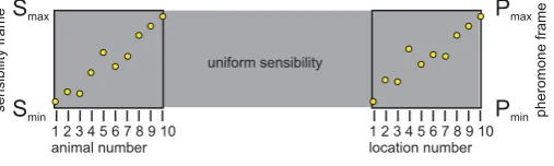
In case of uniformly distributed sensibility and pheromone (Figure 2), the individuals with low level of sensibility can select for start position any location marked with pheromone. The individuals with high sensibility can select for start position locations marked with high level of pheromone and will ignore locations marked with low level of pheromone.
Figure 2: Enhanced sensibility
It is assumed that during a stochastic process within a stochastic environment any deviation could lead to non-uniform changes of the process. The achieved results play a role of deviator. The enhancement of the sensibility urges the individuals to search around the area of the best-found solution from all individuals marked with highest amount of pheromone. This situation appears naturally when the pheromone marks are very different and stochastic generation of the sensibility produces high values. External adding of a constant or a variable to the Smin could make an enforced enhancement of the sensibility (Figure 3).
All the individuals with enhanced sensibility will select and can differentiate more precisely locations marked with a higher level of pheromone and will ignore these indicated with lower level of pheromone.
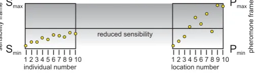
By reducing the sensibility, the individual can be allowed to explore around locations marked with a low level of pheromone. This situation naturally appears when the pheromone marks are very similar and randomly generated sensibility is low. In this case the individuals can select locations marked with low level of pheromone with high probability, which indirectly will decrease the probability for selection of locations marked with high level of pheromone. Subtracting of a constant or a variable from the Smax could make an enforced reduction of the sensibility frame (Figure 3).
Figure 3: Reduced sensibility
The sensibility across all the individuals varies. Different individuals can have different sensibility: Sj Sl for j l, where j and l are numbers of different individuals, j = 1, ..., m,
l = 1, ..., m, m is population size.The sensibility varies also during the optimisation process, and one individual can have different sensibility for different explorations.
Sjg Sjq for g q, where j is a current number of an individual, j = 1, ..., m, m is population
size, g and q are numbers of different explorations, g = 1, ..., G, q = 1, ..., G, G is the limit of exploration.
Free Search performs an adaptive self-regulation of sense, action, and pheromone marks. This adaptive self-regulation is organised as follows. An achievement of better solutions increases the maximal value of the pheromone Pmax. An increase of the Pmax increases the maximal allowed sensibility of the individuals Smax. This is an adaptive regulation between pheromone and sensibility. In fact it is an abstract approach for learning. The sensibility can be considered as high-level abstract cognition about the explored space based on the achieved and assessed result. The individuals do not memorise any data or low-level information, which consume computational resources. By using sense they build cognition about the quality of the search space and in the same time create skills how to recognise further, higher or lower quality locations. Cognition and skills are abstracted from the achieved results. From a philosophical point of view, “abstraction is a form of cognition based on separation in thought of essential for particular purpose entities, characteristics and relationships” [12]. The abstracted cognition influences thinking. The thinking defines behaviour and action. In computer modelling, abstraction influences operation and self-organisation of algorithms. The abstracted cognition defines behaviour of computational process and it’s functioning. The computational process defines action of the computer system and achieved results [12].
Based on relationship between sense and action Free Search implements a computational model of abstraction, cognition, decision-making and action analogous to the processes of perception, learning and thinking in biological systems. This is implemented in the following manner. The better achievements and the higher level of distributed pheromone support enhancement of the sensibility. A higher sensibility does not restrict or does not limit the abilities for movement. It implicitly regulates the individuals’ action in terms of selection of a start location for exploration.
During the exploration walk they continue to do small or large steps according to the modification strategy, without restrictions such as convergence rules. However, enhanced sensibility changes their behaviour. They give less attention to steps or locations, which brings low quality results. They can be attracted with high probability from locations with better quality. If small steps achieve better locations the individuals explore these near locations with higher probability. If large steps achieve better results the individuals explore remote locations with higher probability. In this way sensibility adaptively regulates the action. These regulations can be classified as stochastic and probabilistic. Explicit restrictive rules are not applied. The individuals are allowed to explore any location of the search space and enhanced or reduced sensibility increases or decreases the probability for action. The optimisation process keeps the chances of the algorithm to reach the desired solution anywhere in the space. The experience and knowledge can regulate the probability for particular action less than one and greater than zero but they do not determinate such action with a probability of one (100%) or zero (0%).
2. Visual Tool
Visualization tool for advanced search algorithms (VOTASA) is used for evaluation of selected search algorithms.
The tool generates 3-dimensional visual landscape of selected test functions. Optimization process is animated. Sequentially generated solutions model individuals’ “movement” on the function’s landscape. A three dimensional Cartesian system is displayed around the function, so the user can have a clear view over dimensions and scale.
3. Visual Analysis
3.1. Dependence on Initialisation
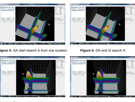
Figure 4: GA start search A from one location Figure 5: GA end of search A
Figure 6: GA start search B from one location Figure 7: GA end of search A
Figures 4, 5, 6 and 7 illustrate dependence on initialisation. Figure 4 shows search process start form single point appropriately located to the global solution and Figure 5 shows successful end of this process. Figure 6 shows search process start form single point located close to local solution and Figure 7 shows end of this process trapped in local hill.
3.2. Divergence
Figure 8: FS start from one location Figure 9: FS divergence within initial walk
3.3. Convergence
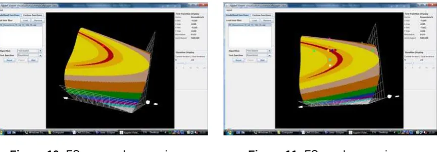
Figure 10: FS approaches maximum Figure 11: FS reaches maximum
Figures 10 and 11 illustrate how process started on Figure 8 continues with approaching and reaching the maximal solution.
Figure 12: DE start on Himmelblau test Figure 13: DE converges to optimal solutions
Figure 12 illustrates how Differential Evolution starts from random locations on Himmelblau test, which has four equal value optima.
Figure 13 then shows how Differential Evolution discovers and converges to three of these solutions within 63 iterations.
3.4. Role of Accidental Events
Figure 16: Use of accidental event Figure 17: FS achieved maximum on Sofia test
Figure 14 shows Free Search start on Sofia test purposefully selected away from the optimal pack. Gradient on more than 90% of this test is in opposite direction to the maximum. Figure 15 shows generation of accidental even within the area of optimal peak. Figure 16 shows other individuals are attracted within the area, and on Figures 17 is visible achievement of the maximum.
4. Discussion
Visual analysis on dependence on initialisation, convergence, divergence and accidental events role in search process confirms previous studies and suggest new conclusions.
Regarding dependence on initialisation most dependant and sensitive to initial start locations are Differential Evolution and Particle Swarm Optimisation. These methods could converge very fast to the global optimum in at least one initial locations are situated appropriately to the global solution. However if initial locations are away from the area of global solution they face difficulties to identify global area. Once trapped in local hill Particle Swarm Optimisation and Differential Evolution converge quickly to the local solution and have no mechanism to escape. Genetic Algorithm is less dependent on initialisation and could start from single location. For Genetic Algorithm when starts form one location search process starts after first successful mutation. Visual analysis suggests that Genetic Algorithm could escape from trapping if an accidental mutation produce location closes the global solution. However probability for such mutation is very low.
According to the divergence observation suggests that Particle Swarm Optimisation and Differential Evolution could slightly diverge on initial stage of the process. In the middle and in the end of the search process Particle Swarm Optimisation and Differential Evolution shows narrow convergence. Visual analysis confirms that Free Search keeps good divergence abilities during the entire search process.
Regarding convergence visualised search processes clearly confirm that Particle Swarm Optimisation and Differential Evolution have excellent convergence abilities. Genetic Algorithm also demonstrates very good convergence. Free Search has no convergence rule and this is visible. Its ability to discover global solution is based on abstracted knowledge from previous iterations, which reflect on its abilities to avoid trapping and facilitate escaping from trapping.
generate accidentally remote locations is restricted by their modification strategies to zero. Visualisation of the Free Search process confirms that it is cabala to generate accidentally remote locations during the whole search process. If good location is generates close to the end of the search process precision of the result could be low. However in order to reach better precision, utilising Free Search ability to start from single location, the achieved result could be used for start location for a next run.
Visual analysis helps to identify that Norwegian test [12] has maximum higher than 1.0. For 10 dimensional version of this achieved result is f10 = 1.0000056276962146 and corresponding variables are presented in Table 1.
Table 1. Norwegian test variables for 10 dimensional results
x0 = 1.0001125410314771 x1 = 1.0001125413709611 x2 = 1.0001125411045073
x3 = 1.0001125410947156 x4 = 1.0001125411117688 x5 = 1.0001125409284484
x6 = 1.0001125411975889 x7 = 1.0001125410082294 x8 = 1.0001125410497957
x9 = 1.0001125411752061
Visual analysis shows how balance between divergence and convergence helps to resolve successfully global optimisation problems. Uncertainty in Free Search supports the balance between divergence and convergence and in fact excludes typical for majority Evolutionary algorithms dilemma – Exploration versus Exploitation [7] where algorithms are unable to abstract knowledge from current search process or to utilise this knowledge if exists to improve further behaviour.
Good examples for abstraction of knowledge from the search process and utilisation of this knowledge are numerical tests where optimal value is unknown such as Bump test [8]. When optimum is unknown selection of appropriate initial location is difficult or impossible. This highly applies for real world tasks and optimisation problems. So that search algorithms, which are dependent on initialisation heed special positioning of initial population without any guarantee. Initialisation becomes even harder when the objective function variables number is high. In such cesses relation of large population increases period of search and for time consuming objective functions search process becomes infeasible.
In distinction from these methods Free Search does not depend on initialisation. It could start form one location and diverge in few steps across the search space. This is visible form Figures 8, 9, and 10. In contrast to stochastic search for appropriate initial position Free Search abstracts knowledge from explored accidental (stochastically) locations, then learns this knowledge and use it to improve its further behaviour [10]. These abilities are best visible on Figures 14, 15, 16 and 17.
As additional illustration on multidimensional search space, which cannot be visualised Free Search is tested on 200 dimensional version of Bump test [8]. Achieved result in June 2012 before OMCO NET - 2012 conference is: f200 = 0.85066363874546513. Constraint for this value is: px= 0.75000000001700473.
Corresponding to this result variables are presented in Table 2.
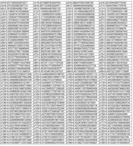
Table 2. Bump test variables for 200 dimensional results
x0=9.4317265092875271 x1=9.4210880763449794 x2=6.2882470551006726 x3=6.2812044305775245 x4=6.2741502992387712 x5=6.2671333083052971 x6=3.1689464500548583 x7=3.1654470461737678 x8=3.1619395428821764 x9=3.1584654487855133 x10=3.1549887585381216 x11=3.1515052609245462 x12=3.1480514316348942 x13=3.144592385248107 x14=3.1411665208632975 x15=3.1377256453531199 x16=3.1342874197299722 x17=3.1308682053155081 x18=3.1274554202686256 x19=3.1240551403195638 x20=3.1206397745048395 x21=3.1172452805912063 x22=3.1138450849729966 x23=3.1104547305099155 x24=3.1070832311300736 x25=3.1036959150231214 x26=3.1003096268012658 x27=3.0969346627763605 x28=3.0935597373930599 x29=3.0901843874090842 x30=3.0868198721408615 x31=3.0834499576245431 x32=3.0800848219433044 x33=3.0767286653290187 x34=3.0733526058628713 x35=3.0699987823771764 x36=3.0666258516333507 x37=3.0632720102951976 x38=3.0598966938543795 x39=3.056530747298678 x40=3.0531402834188994 x41=3.0497919194950507 x42=3.0464144290947432 x43=3.0430407269387443 x44=3.0396564701050011 x45=3.0362606850701988 x46=3.0328889354156199 x47=3.0294878068600708 x48=3.0260868470445264 x49=3.0226970898753449 x50=3.0192938974016523 x51=3.0158656704071416 x52=3.0124692389801191 x53=3.0090220962794261 x54=3.0055937860424233 x55=3.0021473589341481 x56=2.9987124259525304 x57=2.9952468184703789 x58=2.9917779650003822 x59=2.9883074400256104 x60=2.9848201306512165 x61=2.9813333782210765 x62=2.9778122424860944 x63=2.9743090676481345 x64=2.9707730736866949 x65=2.9672348176413172 x66=2.9636847955273784 x67=2.9601062040242381 x68=2.9565227981730566 x69=2.9529188126611881 x70=2.949321676614483 x71=2.9456856440913848 x72=2.9420258470166796 x73=2.9383818720050225 x74=2.9347045145772901 x75=2.9309963260492711 x76=2.9272779930565633 x77=2.9235334986374415 x78=2.9197768976239793 x79=2.9159920376725164 x80=2.9122020062441676 x81=2.9083602523092282 x82=2.9045094322369045 x83=0.45823984817375735 x84=0.45774089710037869 x85=0.45727114217197029 x86=0.4567745894309917 x87=0.4562951728187824 x88=0.45580577745518042 x89=0.45534177489250671 x90=0.45486045054327734 x91=0.45439602845627802 x92=0.45394310840640006 x93=0.4534702935383077 x94=0.4529999847765222 x95=0.45253467706979733 x96=0.45205813151398533 x97=0.45163461981247027 x98=0.45116993319532678 x99=0.45072212587173699 x100=0.45025372360371446 x101=0.44980480403796747 x102=0.44935699125401113 x103=0.44892267440206884 x104=0.44846630677602395 x105=0.44803663148901179 x106=0.44760106190153104 x107=0.44716738095279651 x108=0.44669963065345109 x109=0.446274123158933 x110=0.44585074831078803 x111=0.44539938407422552 x112=0.44498965251514611 x113=0.44458571277670311 x114=0.44413350683067765 x115=0.44371510577426843 x116=0.44329443469773994 x117=0.44286821129784115 x118=0.44245267787636511 x119=0.44205484519500648 x120=0.44163007466742993 x121=0.44120855371288265 x122=0.44081135789805459 x123=0.44038286798602383 x124=0.43998590163931056 x125=0.43958017705749719 x126=0.43916474548458379 x127=0.43876240741271488 x128=0.43837501452723415 x129=0.43796220309859185 x130=0.43757082525431978 x131=0.43718316066159979 x132=0.43678232263091576 x133=0.43638572567134154 x134=0.43601937796054058 x135=0.43560927575532765 x136=0.43521481062800438 x137=0.43484601432010311 x138=0.43444614837081474 x139=0.43405866650450076 x140=0.43369265901309439 x141=0.43330904830153699 x142=0.4329369251673581 x143=0.43254129852963724 x144=0.43215764564206566 x145=0.43179115637484472 x146=0.43140938352389718 x147=0.43103236473890894 x148=0.43067293713980515 x149=0.43031035434332254 x150=0.42992659626446544 x151=0.42956155047094335 x152=0.42918633562991876 x153=0.42881073599387187 x154=0.42846587868984493 x155=0.42809489894581787 x156=0.42772868753273241 x157=0.42738075957025207 x158=0.42704045925640788 x159=0.426657402002658 x160=0.42631824711613514 x161=0.42594983416198534 x162=0.42561228588155675 x163=0.42524880923746006 x164=0.42489999598120565 x165=0.42454938919611024 x166=0.42420793755776337 x167=0.42385506320185307 x168=0.42352014710422675 x169=0.42316372587208445 x170=0.42281936413544152 x171=0.42247821548464565 x172=0.42214409184863272 x173=0.42180508824841179 x174=0.42145599428238661 x175=0.42110540808126568 x176=0.42076842458400371 x177=0.42043315088331829 x178=0.42010917271001941 x179=0.41979625020274952 x180=0.41946151902511214 x181=0.41911049740812506 x182=0.41878042265486326 x183=0.41845325638208147 x184=0.41813241449989075 x185=0.41781316082099201 x186=0.41746717297257324 x187=0.41716175933695726 x188=0.41681473517720607 x189=0.41651618484573272 x190=0.41617618429311293 x191=0.4158466491643748 x192=0.41553632974871946 x193=0.41520773200359601 x194=0.41489921822492909 x195=0.41456812526745412 x196=0.41424967110372368 x197=0.41393940653707634 x198=0.41362772347405607 x199=0.41332913145585537
5. Conclusion
Further research could focus on visual evaluation of other methods and integration with computer aided systems which relay on optimisation.
Acknowledgement
Preparation of this paper is supported by Southampton Solent University, Research and Enterprise Fund, Grant 516/17062011.
References
1. Angeline P., 1998, Evolutionary Optimisation versus Particle Swarm Optimisation: Philosophy and Performance Difference, The 7-th Annual Conference EP, San Diego, USA. 2. Eberhart R. and Kennedy J., 1995, Particle Swarm Optimisation, Proceedings of the 1995 IEEE International Conference on Neural Networks, Vol. 4, 1942-1948.
3. Eberhart R., and Shi Y., 1998, Comparison between Genetic Algorithms and Particle Swarm Optimisation, The 7-th Annual Conference on Evolutionary Programming, San Diego, USA.
4. Eshelman L. J., and Schaffer J. D., 1993, Real-coded genetic algorithms and interval-schemata, Foundations of GA 2, Morgan Kaufman Publishers, San Mateo, pages (187-202). 5. Goldberg D.E., 1989, Genetic Algorithms in Search, Optimisation, and Machine Learning, Addison Wesley Longman Inc. ISBN 0-201-15767-5.
6. Hedar A.R., 2010, Global Optimisation, Kyoto University, http://www-optima.amp.i.kyoto-u.ac.jp/member/student/hedar/Hedar_files/TestGO_files/Page2376.htm, last visited 02.06.10 7. Holland J., 1975, Adaptation in Natural and Artificial Systems, Uni. of Michigan Press. 8. Keane A. J., 1996, A Brief Comparison of Some Evolutionary Optimization Methods, In V.Rayward-Smith, I. Osman, C. Reeves and G.D. Smith, J. Wiley (Editors), Modern Heuristic Search Methods, ISBN 0471962805, pp. 255-272.
9. Penev K., and Littlefair G., 2005, Free Search – A Comparative Analysis, Information Sciences Journal, Elsevier, Vol. 172, Issues 1-2, pp. 173-193.
10. Penev K., 2008, Free Search of Real Value or How to Make Computers Think, Alexander Gegov (Editor), St. Qu publisher, April 2008, ISBN 978-0955894800, UK.
11. Price K., and R. Storn, 1997, "Differential Evolution", Dr, Dobb's Journal, Vol. 22(4), pp. 18-24.
12. Shi Y. and Eberhart R. C., 1998, Parameter Selection in Particle Swarm Optimisation, Evolutionary Programming VII (1998), LNCS, Vol. 1447, pp. 591-600, Springer.
13. Storn R. and Price K., 1995, Differential Evolution – A simple and efficient adaptive scheme for global optimisation over continuous spaces, TR-95-012, International Computer Science Institute, 1947 Center Street, Berkeley, CA 94704-1198, Suite 600.
14. Weisstein E., Global Optimization, WolframMathWorld,
http://mathworld.wolfram.com/GlobalOptimization.html last visit 02.06.12
15. Wolpert D.H., and W.G. Macready, 1997, No Free Lunch Theorems for Optimisation, IEEE Trans. Evolutionary Computation, Vol. 1(1), pp. 67-82.