Operation Research in Computer Science: a
Case Study
Sadhana Chandra#1, Rahul Karmakar*2
#1
MSc final year student, Department of computer science, The University of Burdwan, W.B, India. *2
Assistant Professor, Department of computer science, The University of Burdwan, W.B, India.
Abstract — Computer science and Operation Research (OR) are interrelated since their origin, each contributing to the dramatic advances of the other. The main idea of operation research-based modelling in computer science applications is the systematic approach to deal with the problem and get the optimized solution. This is one of the best platforms where we get the best knowledge through profit and loss concept. This study is aimed to find the minimum cost and expected time to finish a project. Operation Research also represents a clear idea about co-operation between intelligent relations with decision making. The optimization models are very useful in computer science, especially in software engineering and computer network domains. A system model can be built and mathematically prove by O.R models. The main overview of Operation Research is to give the perfect solutions to win a war without fighting it. The implementation of O.R. is mainly depended on the person who provides the solution and the person who use the solutions. In this paper, we try to discuss and find the research directions of optimization models in computer science domains.
Keywords — Linear programming, Inventory management, Game theory, Queuing model, Network model,
Markov model, Transportation model.
I. INTRODUCTION
The term of ‗Operations Research' was coined in 1940 by McCloskey and Trefethen in a small town of Bawdsey in England [3]. Mainly, Operation Research concept comes from during II world war [13]. It is a Management science concept that came into a military context. Military context means, how to maximize the resources (food, medicine etc) in the certain period of time. Consequently, resources are not properly allocated to all over the army persons, to overcome that situation OR techniques are used for proper allocation of resources. After seconds world war the scientists who had been active in military war problem turned their attention to the possibilities of applying the same approach to civilian problems. In term of application the first civilian problem applying the large profit-making corporation. For examples (petroleum companies first to make regular uses of linear programming on a large scale for production planning).So, it was logically adopted that the profit and loss concept hugely dependents on O.R. terminology [8]. In the earlier time the concept of O.R. only acceptable by the large companies, but later when inventory, allocation, replacement, scheduling etc technique come on that time this method also used in small companies. Many applications of Operations Research techniques can easily apply through the computer because it is one of the best platforms where we use of the computers and made it possible to apply any O.R. techniques for practical decision analysis. Therefore many colleges and universities introduced O.R. their curriculum. Consequently, Operations Research generally useful for computer science, mathematics, economics, engineering, business management etc [14]. O.R. creates multidisciplinary feature and application in various fields; it has a bright future to improve our society, some of the daily life problem which is hospital management, energy conservation, environmental pollution etc that have been solved by O.R. It can also contribute to improvement in the social life and area of global needs.
II. DIFFERENT TYPES OF OPTIMIZATION MODEL
We try to discuss different types of optimization models in this section.
A. Linear Programming Model
programming model consists of some following condition: Study the given problem and find out the decision variable of the problem (the major task of the given problem declared as a decision variable). After finding the decision variable designate them by symbols xi (i=1, 2, .n). And State the feasible condition which generally is
xi>= 0 for all i. Identified the constraints variable in the problem and express them a linear equation. Finally,
identified the objective function and express it as a linear function of the decision variable. So that the general formulation of LLP following as First finds out the decision variable x1, x2…..xn to maximize and minimize the
objective function. Z= c1x1+c2x2+……. +cnxn ...(i) And also satisfy p constraints.
a11x1+a12x2+………. +a1nxn….b1
a21x1+a22x2+………. +a2nxn….b2
ai1x1+ai2x2+…………+ainxn….bi ….(ii)
am1x1+am2x2+………...+amnxn… bm [3]. Where the constraints form is either equality (=) and another form is
inequality (means <= or >=) and finally satisfy the non-negative restrictions (means we can produce few amount of the product so that it cannot be a negative). x1>=0, x2>=0…..xn>=0…(iii)The LPP can be expressed in the
matrix form as follows: Maximize or Minimize Z= cx (objective function). Subject to, Ax (<=, =, >=) b (Constraint equation). b>0, x>=0 non negative restrictions.
Where, Ax=b, A= (aij)m*n = (a1, a2, a3...an) aj=(a1j,a2j,a3j….amj)T , x= (x1, x2, x3 ,…..., xn), c= (c1, c2,
c3 ,……, cn), b= (b1, b2, b3,…..,bm)T[3]. So we can easily solve any complex problem using this mathematical
technique of LPP. The application of the linear programming problem extensively used in computer science in such different fields as optics, cryptography, electric circuit, computer graphics, dynamic programming, data structures (find out the shortest path) and 3D game programming is the most visible and obvious application, as well as matrix calculation, as the most important applications. So that, Linear Programming has a great play role in computer graphics, data compression. A new neural network for solving general linear programming problem and the most important advantages of the neural networks are heavily used in parallel processing and fast convergence [2]. Linear programming is the most important area in computer science with a manifold application. Therefore, computer science intricately linked with the linear programming problem through the detonating growth of parallel processing and computing a very large scale
.
B. Inventory Model
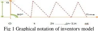
An inventory model can be defined as a mathematical model to determine the optimum solution [4, 19] and also determine the inventory model can be defined as a stock means how to do we have properly managed the stock and proper usages. Management means proper usage of any item just like that efficiency and effectiveness. It is a physical stock of well kept for future use. Inventory management means to have a control over the stock by the manager so that there the proper usage of material is possible with at least wastage. When we purchasing materials the total cost of those materials are some of the: 1) purchasing cost 2) ordering cost 3) carrying a cost. The original cost of the product which is set by the manufacturer with certain profit. The purchasing cost will be considered with discount on any purchases of certain quantity that is called the purchasing cost and Ordering Cost It is a fixed cost associated with obtaining the goods through placing of an order or setting up a machinery before starting the production as well as Carrying Cost associated with carrying and holding the goods in stock is known as carrying cost. So that, before the purchasing of any product we want to know that the carrying cost is not excessive come in the futures. If we order an item in a single purchasing model then the carrying cost is to minimize the total average variable cost per unit time. Finally, we can say that a minimum number of ordering cost, carrying cost and purchasing cost is called EOQ(Economic Order Quantity) means the minimum number of quantity and also economic which is ordered by the user. The basic mathematical situation can be shown in inventory time diagram. Therefore, we can better understanding. [4].
Fig 1 Graphical notation of inventory model
It assumes that after each interval of time t, the quantity Q is produced or supplied the entire time period; say one year [4]. Now then denotes the total number of quantity produced during the one year, then we have written nt= 1 and D = nQ, n = Q/D [5].It may be clear that total inventory over the time period t days so the area of the first triangle= (1/2*Qt) [5]. Thus the average inventory at any given day in the t period is: (½ Qt)/t = ½*Q [5]. The average amount of inventory in each interval of length t during the entire period so the annual inventory carrying or holding cost is given by f1 (Q) = ½ QC1, Annual set up or ordering cost associated with the size Q
are given by [5, 3] f2 (Q) = nCs = DCs/Q. Since the minimum total cost occurs where the ordering cost and the
carrying cost are equal, we must have written f1 (Q) = f2 (Q). So that, ½ QC1 = DCs/Q. Hence, the optimum
value of Q is =√ (2DCs/C1)
Q = √ (2DCs/uI) where (I = Inventory cost and u is per unit time). Therefore optimum number of orders
placed per year, n = D/Q = √ (DC1/2Cs) [5, 3]. So the optimum length of time between orders, t = T/n = T √
(2Cs/DC1) [5, 3]. When T (total time of horizon) in one year. Therefore, total annual cost is given by CA = f1 (Q)
+ f2 (Q) = ½ QC1 + DCs/Q = √ 2DC1Cs [5, 3]. Therefore, we can easily say that the application of the inventory
model extensively used in computer science in such different fields as Intelligence technique, neural networks, intelligent agent system and Cellular Automata etc. Inventory Model has a great play role in Computer Science to find out the solution in minimum time with minimum travels and design the minimum number of state to find out the optimum solution or another side a computerized inventory management model creates an inventory management software. The main objective of this software for tracking the inventory levels, orders, sales, and deliveries. It can also use in the manufacturing industry to create a work order, bill of materials and other production related document.
C. Game Theory Model
Game theory was established the great mathematician John von Neumann proposed a non-cooperative zero-sum game between two people [6, 7, 13]. It uses business organization and other different fields to find out what types of strategy are followed by the competitor as well as other competitor follow that strategy and developed its own strategy [24]. Therefore, a competitor belongs to the down position of the other competitor. Simple example: Pepsi and coca-cola both is the competitor in each other. If coca-cola is going onwards than the Pepsi, so the coco-cola see that and what types of strategy are available in the Pepsi. Consequently, coca-cola understands it and what type of new product is come through the Pepsi so that the coca-cola tries to launch a new product over Pepsi. Different types of game strategy are available in game theory, those are following, it is called two persons zero-sum game because only two people can play at a time with each other, and zero-sum means the algebraic gains and loss of all players is zero [6]. Maximin and Minimax principal: This method is used to find out the optimal strategy between two players. In this method, the problem is represented as a matrix form. This matrix is said to be pay off matrix [8, 7]. One side of the matrix denoted the characteristics of one player and the other side of the matrix are represented the characteristics of another player. Minimax means to find out the minimum value from every row and then select the maximum one (means selects those items where player one gain more profit). Maximin means to find out the maximum value from every column and select the minimum one (means the other player try to decrease his loss). When minimax and maximin method generated the same value is called saddle point [7, 8, 9].Dominance property: - In this property, the problem also represented in matrix form, which is called pay off matrix.The main goal of this property to reduce the matrix size and find out the optimum solution [5]. For reducing the matrix size this method follows some rules: a. If all elements of a row, say kth, are less than or equal to the corresponding elements of any other row say rth, the kth
row is dominated by rth row [5]. b. If all elements of a column, say kth, are greater than or equal to the
corresponding elements of any other column say rth, the kth column is dominated by rth column [5]. c.
Dominated rows or columns may be deleted to reduce the size of payoff matrix [5, 24]. Graphical Solution of (2*n) and (m*2) Games: - It is clear that if one player has only two Strategies, the other player will also use two strategies [24]. Hence, we can find which of the two strategies can be used. Game theory is one of the most popular concepts that are using in computer science. In very short time game theory is to gain very attraction to the computer science. It has the endless application in computer science. The monumental applications of game theory in robotics, cloud computing, Spot pricing, network security, machine learning, social network, recommendation system and resource management system [6]. Cloud computing is one of the most important aspects of computer science. In cloud computing, game theory is used to an interaction between cloud providers whose tasks have minimized the cost using a maximum number of resource utilization. In such a situation game always set up a utility function that will eventually steer game-play together an equilibrium state. Where no players can changes their strategy that state where all players are balanced. In similar case game theory applied in network security. This is one of the most important aspects of computer science. In computer networking user can access or send the maximum number of information in the minimum number of time and also the security must be preserved for data accessibility. The Network also provided the hidden security for the huge amount of network data. In general game, the theory provides a quantitative and analytical technique for describing and analyzing interactive decision scenarios in the computing system.
D. Network Model
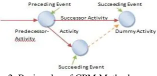
finish the project. Examples of projects include constructions of a bridge, highway, power plant, construction of a building etc [15].CPM identified what types of task are involved in the project, time estimate of every activity [16], the time taken to complete the whole project and completing the project on time. Example:- constructor house(CPM also called repeated nature because a builder can easily say that with his experience or knowledge to give the idea to complete a building, CPM completes a task in a proper time for that reasons builder can easily calculate the cost).On the other hand, PERT (Program Evaluation and Review Technique) also called not repeated nature [16] means if any work is developed firstly than it is called part, it means cannot give the proper idea to completed a task in proper time, therefore, can't easily identify the cost. Some basic rules are used to CPM (Critical Path Method):-Every link does not cross to each other. Apply always straight arrows. No event can occur until the previous event has been completed. Always use arrows from left to right. Dummy state include only when it is necessary [16]. Given the following network diagram for better understanding
Fig. 2 Basic rules of CPM Method.
Activity time is the main time of the network which is start from starting of the network and carry forward up to end of the network. Now use the following notation to design the CPM. (i, j) = Activity with a tail event I and head event j.Tij = Estimated completion time of activity.ESij = Earliest starting time of activity.ESij = Earliest
finishing time of activity.LSij = Latest starting time of activity.LFij = Latest finishing time of activity. Forward
pass completion yields the earliest start and earliest finished of the network [5, 3, 7, 8]. Hence, the completion will start the starting nodes and goes towards the ending node let Zero be the starting time of the project. Earliest start time is the earlier possible time when the activity is can begin [17]. Let us consider that the all activity can be started their earlier start time and the earlier finished time is the earliest start time + activity time and finally earlier start time of the event is the maximum of the earlier finished time of all the activities [7,8,5,3].Similarly, backward process is vice versa of the forward pass computation. Finally, latest event time is the minimum of the latest start time of all activity. After performing the all computations means to find out the earliest start time and latest completion time of the network in which place of the n/w both time is same from start to end node that path is called CPM. On the other hand, PERT also called not repeated nature means if any work is developed firstly than it is called part, it means cannot give the proper idea to completed a task in proper time, therefore can't easily identify the cost. Consequently, the PERT system is based on three-time estimates these are 1) Optimistic time (t0):- This is the shortest completion time if all goes well [7, 5, 8]. Pessimistic time (tp):- This is
the longest completion time if things go bad conditions [7, 5, 8]. Most likely time (tm):- The completion time we
would expect under normal conditions [7, 5, 8].
Fig. 3 Time distribution curve
PERT procedure some different stages those are described below: First of all, draw the project network and compute the expected time referred to as average or mean time and indicated 50% chance of completing the activity within this time. It is denoted by te = t0 + 4tm + tp /6 and also calculated expected variance is the measure
of uncertainty of the probability is to help to complete the specific tasks within the expected time [7]. Variance (∂2
) =(tp – to/ 6)2 as well as compute the earliest start, earliest finish, latest start, latest finished time and total
float of each activity and then find out the critical path and identify their critical activity, also find the project length variance ∂2
therefore we calculated standard normal variable(p) = (Ts - Te)/ ∂ [7], where Ts is the
scheduled time to complete the project, Te is the project mean duration and ∂ is the expected standard derivation
computer science but also hugely used in the in the Engineering, mathematical, and economics etc. These case studies models are a powerful teaching technique and an effective way to learn about how to make decisions on software projects and how to analyze and learn from real-life scenarios.
E. Queuing Model
A common situation occurring in everyday life is that of the queuing or waiting in a line [11]. Some example of queuing model is a bus stop, ticket booths, doctor clinic or hospital [12], bank counters, traffic light, car washing center, telecommunications etc. Usually queuing theory is the mathematical study of waiting lines. Example:- many customers arrive at a service counter and servicing your car. Therefore calculated how many customers or cars are present in the queuing system and how many time to take a car servicing center and also calculated the frequency of each and every car arrive at a service center. Hence, we can easily understand queue discipline is a parameter that explained how the customers arrive at a service facility. Therefore, generally, the four types of customer behavior are present in the queuing theory those
are:-Balking means if the customer nothing joined and leaves the queue or the queue is too long so he may decide not to enter queuing system [3, 5]. On the other hand, a customer may enter the queue but the queue is lost patience and the customer decides to leave the queuing system, in this case, is said to be reneging, sometimes we can say it like ticket counter when there are one or more queue, customer may move one queue to another queue for his personal economic gains, that is called jockeying [3, 5]. The queuing models are classified as follows:
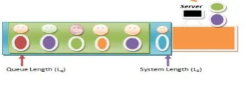
Model 1: (M/M/1): (∞/FCFS):- One queue and one server use. This denoted first M is exponential inter-arrival and second M is exponential service time, single server, infinite capacity and first come first serve service discipline [10].
Fig. 4 Queuing System
Some basic formulas are uses to find out the different problem with this model [8]:- ƥ = €/µ (where € is the mean arrival rate or µ is the mean service rate) [11]. Lq = ƥ2/(1- ƥ)[where ƥ is the utilization factor or find out the
total time for the server is busy and Lq means an average number of customer in the queue but that customer
was not counted who is present in the first position in of the queue). LS = ƥ / (1- ƥ) [where Ls means an average
number of the customer waiting in the system]. n = number of the customers in the system. Pn = probability of n
customer in the system. Wq = Lq/ € [where waiting time in the queue].Ws = Ls/ € [where waiting time in the
system]. N = maximum number of customer allowed in the system. S = number of service channel.
Model 2:(M/M/1):(N/FCFS):-This model denoted first M is exponential inter-arrival and second M is exponential service time, single server, finite(Limited) capacity and first come first serve service discipline [18]. Ex: - limited seating arrangement in a restaurant. Hence, the service system can accommodate N number of customer only (N+1) number of the customer is not allowed in the queue [3]. So we can know that probability of having one customer in the queuing system so that, P1 = (€/µ)* P0. Similarity, probability of having N number
of customer (means n = 0, 1, 2, 3,…,N) so that the equation is: - Pn = (€/µ)n* P0 [where n<=N]. If some of the
probability of the Nth number of the customer is 1. Then the equation:- Or, ∑n=0N pn = 1 Or, ∑n=0N (€/µ)n P0 = 1 Or,
P0 ∑n=0N (€/µ)n = P0 ∑n=0NPn= P0 [1+ ƥ+ ƥ2+ …..+ƥN] = P0 [(1- ƥN+1)/1- ƥ]. So the probability of having no
customer in the finite single server is P0 [(1- ƥN+1)/1- ƥ] [5]. Model 3: (M/M/S): (∞/FCFS):- It model takes the
F. Markov Model
Markov chain models developed by the Russian mathematician Andrei A. Markov in 1905 [3], are a particular class of probabilistic model known as stochastic processes [20], in which the current state of a system depends on all of its previous states. But in Markov model, the current state of a system depends only on it's the immediately preceding state [5] and hidden Markov model (HMM) target tracking problem (like aircraft). HMMs are widely used to our real-world systems (Like graph matching) [21]. The implementation of this model, algorithm and application outlines recent develop. This model basically used in queuing sequence, internet, reverse logistics, inventory system, bio-informatics, DNA sequence, genetic network, data mining, pattern recognition [20], and many other practical systems. The main fundamental method of the MARKOV CHAIN process is to take two states which are undergoing transitions from one state to another [22], between a finite and countable number of possible state, it is one of the infinite numbers of process where the next process depends only on the current process and not on the sequence of events that preceded it. This kind of memory-less is called MARKOV property. Therefore, Markov chains to sample from very large data sets. Markov chains one of the most important concepts in computer science. It can be represented as a directed graph with constant nonnegative edge weights. The Markov property that the future states depend only on the current state and the example are kept to basic day to day operations for the reader to understand and apply.
G. Transportation Model
This model was first developed by Hitchcock [23]. This model aims to get the minimum transportation cost depending on the demand and supply. We get the initial basic feasible solution (IBFS) using North West (NW) corner method, Matrix minimum or least cost method, and Vogel's approximation (VAM) method. A problem is formulated in the tabular form. The problem may be balanced or unbalanced in nature. If the sum of demand is not equal to the sum of supply then we call it an unbalanced problem and can be converted into the balanced problem with dummy moves. Modified distribution method (MODI) is an optimization technique used to get the basic feasible solution (BFS) and find the final optimal basic transportation cost [8, 5]. Assignment problem is the variation of transportation problem to get the minimum assignment cost. Another side we explain traveling salesman problem is a variation of the transportation problem. A salesman has to visit n number of cities. He wishes to start a particular city, visit exactly each and every city in once time and return to his starting city. This model is the traditional computer science approaches is to find out the minimum to minimum shortest circuit path through an optimization. Different fields use in computer science such as Artificial Immune System, genetic algorithm, neural network etc. In this problems are coming into the real-life problem and many kinds of researchers after this type of method are particularly attractive in the fields of the Artificial Intelligence and algorithm design subject uses in the computer science. The traveling salesman problem is an NP problem. Therefore, in this case, study generally solved through the practical or mathematical solution.
Discussion and Study
In this paper, we try to discuss different areas that lead many directions for future work. Some directions simply propagate to computer science through our work. We study optimization models and try to find the research gap in the field of computer science. We summarize our comparative study and application domains of the optimization models in a table shown below.
TABLE I
Comparison of different Optimization models
Serial No
Optimizatio n Model
Inventor Application Domain Cost Year of
Invention
Useful Components
1 Linear Model
George B Dantzig and Kantorovich
It is widely used the field of optimization for several reasons such as business, service, industry etc.
Given a System minimize cTx subject to AX<=b, x>=0. 1939 to 1947
The variables are also subject to the condition in the form of Linear equation.
2 Inventory Model
J.O.Adimoha‘s It is considered an asset and retail store so the accountant must consistently use a valid method for assigning costs to inventory in order to record it as an asset.
Since inventory is rather expensive. Not finding the proper invention time.
It serves different product which prescribe maximum And minimum inventory.
3 Game Model J.Von Neumann
It is mainly used in economic, political, science, as well as logic,
It depends upon the current
1944 to 1970
computer science, biology. situation of the problem
strategy b/w two or more
the player in a situation Constraining set rules and outcomes. 4 Queue
Model
Agner.Krarup. Erlang
It is a mathematical study of waiting lines and the ideas have seen including telecommunication, traffic engineering, shops Cost provide the service 1878 to 1929 Input source generates customers, service discipline, service mechanism etc.
5 N/W Model PERT was developed U.S.Navy company and CPM was developed E.I.DUPont company
CPM and PERT both are project management techniques so that it is needed of western industrial, military establishment to plan, schedule and control complex project. Cost mainly estimates for each activity PERT and CPM both are basically started at the same time in 1956 to 1958
Event and Activity
6 Transportati on Model
F.L.Hitchcock, T.C.
Koopmans, G.B Dantzig.
It is the simplified version of the simplex technique such as find out the shortest path. Uses minimum cost to solving the transportati on problem 1941(Hitc hcock) 1949(Koo pmans) 1951(Dant zig). Solving problem involving several products, source and Several destinations of the product. 7 Markov
Model
Andrei A.Markov
Used in modelling many practical problems such as queuing system, manufacturing system. Cost is dependent on the product feature
1905 Modelling categorical data sequence.
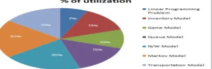
In this paper, we also try to give the brief concept of optimization techniques. We find these models are very useful to get the minimum cost and time. These models are linear and nonlinear in nature. We find that homogeneous Markov chain is sensitive in the reflection of development and changes of process. Since Operation Research is hugely propagation to its own different optimization technique so that we discuss utilization factors of the models.
Fig. 3 utilization of different optimization models
From the above pie chart, we get an idea of utilization factor of every model in different real-world application domains. All utilization factors are our assumptions and are based on our study.We think 7% is utilized for LPP, 13% for inventory model, 10% is used for game theory model, 15% is used for queue model, 20% is used for n/w model, 20% is used for Markov model and 15% is used for transportation model.
.
III.CONCLUSIONS
great roles in computer science domain. This optimization techniques help the designers to get the optimized solutions.
ACKNOWLEDGMENT
Thankful to Rahul Karmakar sir for support, motivation and useful guidance during this work.
REFERENCES
[1] John.C. Nash, ―THE (DANTZIG) SIMFLEX METHOD FOR LINEAR PROGRAMM,‖ Computing in Science & Engineering, Vol. 2, no.1, pp. 29-31, 2000.
[2] Youshen Xia, ―A New Neural Network for Solving Linear Programming Problems and Its Application,‖ IEEE Transactions on Neural Networks, vol. 7, no. 2, pp. 525 – 529, 1996.
[3] S Kalavathy, "Operations Research," Vikas Publishing House Pvt Ltd, 2013.
[4] G. Fauza, Y. Amer, S. H. Lee, H. Prasetyo, ―A Vendor-Buyer Inventory Model for Food Products Based on Shelf-Life Pricing,‖ Operations and Supply Chain Management, vol. 8, pp. 67-73, 2015.
[5] Kanti Swarup, p.k. gupta, man Mohan, "operations research," Sultan Chand & Sons Publishers, 1977.
[6] He Zhang, Yuelong Su, Lihui Peng, Danya Yao Member,―A Review of Game Theory Applications in Transportation Analysis,‖ International Computer and Information Application(ICCIA), 2010.
[7] Rasajit Bera, Pratap Chandra ray, ―Operation Research & Optimization Techniques,‖ Matrix Educare PVT. LTD Publishers, 2005. [8] J.K.Sharma, ―Operations Research Theory and Applications,‖ Macmillan India Ltd Publishers, 1997.
[9] Mark Rahmes, Kathy Wilder, Kevin Fox, Rick Pemble, ―A Game Theory Model for Situation Awareness and Management,‖Consumer Communications and Network Conference (CCNC) IEEE,pp.909-913, 2013.
[10] Nancy Ambritta P., Poonam N. Railkar, Parikshit N. Mahalle, ―A Queuing Theory-based Modelling for Performance Analysis towards Future Internet‖, India Conference (INDICON), 2014 Annual IEEE.
[11] Fatima Al Qayedi, Khaled Salah, M. Jamal Zemerly, ―Queuing Theory Algorithm to find the minimal number of VMs to satisfy SLO response time,‖ Information and Communication Technology Research (ICTRC), 2015 International Conference on.
[12] M. Egerstedt, Y. Wardi, ―Multi-Process Control Using Queuing Theory,‖ Proceedings of the 41st IEEE Conference on Decision and Control, 2002.
[13] 13. A.RAVINDRAN, DON T.PHILLIPS, JAMES J. SOLBERG, ―OPERATIONS RESEARCH PRINCIPLES AND PRACTICE,‖ Wiley India Publishers, 2000.
[14] Junyi Chen, Pingyuan Xi,"Simulation and Application of Modern Operational Research," The 2nd International Conference on Computer and Automation Engineering (ICCAE), 2010.
[15] W. H. Marlow, ―Mathematics for Operations Research,‖ Dover Publications Inc, 2003. [16] http://NPTEL.AC.IN/NOC
[17] Matthew J. Liberatore, ―Critical Path Analysis with Fuzzy Activity Times,‖ IEEE Transactions on Engineering Management, Vol. 55, no. 2, pp. 329 – 337, 2008.
[18] D.S. Hira, P.K. Gupta, ―Operations Research,‖ S. Chand & Company Ltd Publication, 2014.
[19] Z. Prihar, ―Operations Research: The Inventory Problem,‖ IRE Transactions on Engineering Management, Vol.EM-4, no. 1,pp. 9-12,1957.
[20] Lu Yu, Jason M. Schwier, Ryan M. Craven, Richard R. Brooks, Christopher Griffin, ― Inferring Statistically Significant Hidden Markov Models,‖ IEEE Transactions on Knowledge and Data Engineering, Vol. 25, no. 7, pp. 1548 – 1558, 2013.
[21] Vikram Krishnamurthy, Robin J. Evans, ―Hidden Markov Model Multiarm Bandits: A Methodology for Beam Scheduling in Multitarget Tracking,‖ IEEE Transactions on Signal Processing, Vol. 49, no. 12, pp. 2893–2908, 2001.
[22] Chen Lu, Jason M. Schwier, Ryan M. Craven, Lu Yu, Richard R. Brooks, Christopher Griffin, ―A Normalized Statistical Metric Space for Hidden Markov Models,‖ IEEE Transactions on Cybernetics, Vol. 43, no. 3, pp. 806 – 819, 2013.
[23] Amrit Das, Uttam Kumar Bera, Manoranjan Maiti, "A Profit Maximizing Solid Transportation Model under Rough Interval Approach," IEEE Transactions on Fuzzy Systems, Vol.25, no. 3, pp. 485 – 498, 2017.
[24] A. V. Vasilakos, R. Kannan, E. Hossain, Herbert Gintis, "Guest Editorial Special Issue on Game Theory," IEEE Transactions on Systems, Man, and Cybernetics, Part B (Cybernetics), Vol.40, no. 3, pp. 554 – 558, 2010.