Collaboration Based Multi-Label Learning

(1)

The Thirty-Third AAAI Conference on Artificial Intelligence (AAAI-19)

Collaboration Based Multi-Label Learning

Lei Feng,

1,2

_{Bo An,}

1

_{Shuo He}

3

1_{School of Computer Science and Engineering, Nanyang Technological University, Singapore}

2_{Alibaba-NTU Singapore Joint Research Institute, Singapore}

3_{College of Computer and Information Science, Southwest University, Chongqing, China}

{feng0093, boan}@ntu.edu.sg, [email protected]

Abstract

It is well-known that exploiting label correlations is crucially important to multi-label learning. Most of the existing ap-proaches take label correlations as prior knowledge, which may not correctly characterize the real relationships among labels. Besides, label correlations are normally used to regu-larize the hypothesis space, while the final predictions are not explicitly correlated. In this paper, we suggest thatfor each individual label, the final prediction involves the collabora-tion between its own prediccollabora-tion and the prediccollabora-tions of other labels.Based on this assumption, we first propose a novel method to learn the label correlations via sparse reconstruc-tion in the label space. Then, by seamlessly integrating the learned label correlations into model training, we propose a novel multi-label learning approach that aims to explicitly ac-count for the correlated predictions of labels while training the desired model simultaneously. Extensive experimental re-sults show that our approach outperforms the state-of-the-art counterparts.

Introduction

Multi-label learning deals with the problem where an in-stance can be associated with multiple labels simultane-ously. Formally speaking, letX ∈Rdbed-dimensional

fea-ture space andY={y1, y2,· · ·, yq}be the label space with

qlabels. Given the multi-label training setD={xi,yi}ni=1 wherexi ∈ X is a feature vector and yi ∈ {−1,1}q is the label vector, the goal of multi-label learning is to learn a modelf : Rd → {−1,1}q, which maps from the space

of feature vectors to the space of label vectors. As a learn-ing framework that handles objects with multiple seman-tics, multi-label learning has been widely applied in many real-world applications, such as image annotation (Yang et al. 2016), document categorization (Li, Ouyang, and Zhou 2015), bioinformatics (Zhang and Zhou 2006), and infor-mation retrieval (Gopal and Yang 2010).

The most straightforward multi-label learning ap-proach (Boutell et al. 2004) is to decompose the prob-lem into a set of independent binary classification tasks, one for each label. Although this strategy is easy to im-plement, it may result in degraded performance, due to

the ignorance of correlations among labels. To compen-sate for this deficiency, the exploitation of label correlations has been widely accepted as a key component of effective multi-label learning approaches (Gibaja and Ventura 2015; Zhang and Zhou 2014).

So far, many methods have been developed to improve the performance of multi-label learning by exploring various types of label correlations (Tsoumakas et al. 2009; Cesa-Bianchi, Gentile, and Zaniboni 2006; Petterson and Cae-tano 2011; Huang, Zhou, and Zhou 2012; Huang, Yu, and Zhou 2012; Zhu, Kwok, and Zhou 2018). There has been in-creasing interest in exploiting the label correlations by tak-ing the label correlation matrix as prior knowledge (Har-iharan et al. 2010; Cai et al. 2013; Huang et al. 2016; 2018). Concretely, these methods directly calculate the la-bel correlation matrix by the similarity between lala-bel vec-tors using common similarity measures, and then incorpo-rate the label correlation matrix into model training for fur-ther enhancing the predictions of multiple label assignments. However, the label correlations are simply obtained by com-mon similarity measures, which may not be able to reflect complex relationships among labels. Besides, these meth-ods exploit label correlations by manipulating the hypothe-sis space, while the final predictions are not explicitly corre-lated.

(2)

by experimental results on a number of datasets.

Related Work

In recent years, many algorithms have been proposed to deal with multi-label learning tasks. In terms of the order of label correlations being considered, these ap-proaches can be roughly categorized into three strate-gies (Zhang and Zhou 2014; Gibaja and Ventura 2015).

For the first-order strategy, the multi-label learning prob-lem is tackled in a label-by-label manner where label cor-relations are ignored. Intuitively, one can easily decompose the multi-label learning problem into a series of independent binary classification problems (one for each label) (Boutell et al. 2004). The second-order strategy takes into considera-tion pairwise relaconsidera-tionships between labels, such as the rank-ing between relevant labels and irrelevant labels (Elisseeff and Weston 2002) or the interaction of paired labels (Zhu et al. 2005). For the third-order strategy, high-order relation-ships among labels are considered. Following this strategy, numerous multi-label algorithms are proposed. For exam-ple, by modeling all other labels’ influences on each label, a shared subspace (Ji et al. 2008) is extracted for model train-ing. By addressing connections among random subsets of labels, a chain of binary classifiers (Read et al. 2011) are sequentially trained.

Recently, there has been increasing interest in second-order approaches (Hariharan et al. 2010; Cai et al. 2013; Huang et al. 2016; 2018) that take the label correlation matrix as prior knowledge for model training. These ap-proaches normally directly calculate the label correlation matrix by the similarity between label vectors using com-mon similarity measures, and then incorporate the label correlation matrix into model training for further enhanc-ing the predictions of multiple label assignments. For in-stance, cosine similarity is widely used to calculate the la-bel correlation matrix (Cai et al. 2013; Huang et al. 2016; 2018). Such label correlation matrix is further incorporated into a structured sparsity-inducing norm regularization (Cai et al. 2013) for regularizing the learning hypotheses, or performing joint label-specific feature selection and model training (Huang et al. 2016; 2018). In addition, there are also some high-order approaches that exploit label corre-lations on the hypothesis space, while they do not rely on the label correlation matrix. For example, a boosting ap-proach (Huang, Yu, and Zhou 2012) is proposed to exploit label correlations with a hypothesis reuse mechanism.

Note that most of the existing approaches using label cor-relation matrix are second-order and focus on the hypoth-esis space. Such simple label correlations exploited in the hypothesis space may not correctly depict the real relation-ships among labels, and final predictions are not explicitly correlated. In the next section, a novel high-order approach with crafted label correlation matrix that focus on the label space will be introduced.

The CAMEL Approach

Following the notations used in Introduction, the training set can be alternatively represented byD = {(X,Y)}where

X = [x1,x2,· · ·,xn]> ∈ Rn×d denotes the instance

ma-trix, andY= [y1,y2,· · · ,yn]> ∈Rn×q denotes the label

matrix. In addition, we denote byYj ∈Rnthej-th column

vector of the matrixY(versusyj ∈Rqfor thej-th row

vec-tor ofY), andY−j = [Y1,· · · ,Yj−1,Yj+1,· · ·,Yq] ∈

Rn×(q−1)represents the matrix that excludes thej-th

col-umn vector ofY.

Label Correlation Learning

To characterize the collaborative relationships among labels regarding the final predictions, CAMEL works by learning a label correlation matrixS = [sij]q×q wheresij reflects the contribution of thei-label to thej-label. Guided by the assumption thatfor each individual label, the final prediction involves the collaboration between its own prediction and the predictions of other labels, we thus take the given label matrix as the final prediction, and propose to learn the label correlation matrixSin the following way:

min sij

((1−α)Yj+α

X

i6=j,i∈[q]

sijYi)−Yj

2

2 (1)

whereαis the tradeoff parameter that controls the collabo-ration degree. In other words,αis used to balance thej-th label’s own prediction and the predictions of other labels. Since each label is normally correlated with only a few la-bels, the collaborative relationships between one label and other labels could be sparse. With a slight abuse of notation, we denote by Sj = [s1j,· · ·, sj−1,j, sj+1,j,· · · , sqj]> ∈

R(q−1)thej-th column vector ofSexcludingsjj(sjj = 0). Under canonical sparse representation, the coefficient vector

Sjis learned by solving the following optimization problem:

min

Sj

k(1−α)Yj+αY−jSj−Yjk2₂+ ˆλkSjk₁ (2)

whereλˆcontrols the sparsity of the coefficient vectorSj. By properly rewriting the above problem and settingλ= ˆλ/α, it is easy to derive the following equivalent optimization problem:

min

Sj

kY−jSj−Yjk 2

2+λkSjk1 (3)

Here, this problem aims to estimate the collaborative re-lationships between thej-th label and the other labels via sparse reconstruction. The first term corresponds to the lin-ear reconstruction error via`2 norm, and the second term controls the sparsity of the reconstruction coefficients by us-ing `1 norm. The relative importance of each term is bal-anced by the tradeoff parameter λ, which is empirically set to ₁₀₀1 Y_j>Y−j

(3)

al. 2013; Huang et al. 2016; 2018), only pairwise relation-ships are considered, and the relationrelation-ships between one label and the other labels are separated. While for CAMEL, since the final prediction of each label is determined by all the pre-dictions of other labels and itself, the relationships among all labels are exploited in a collaborative manner. Which means, the relationships between one label and the other labels are coordinated (influenced by each other). Therefore, CAMEL is a high-order approach.

Multi-Label Classifier Training

In this section, we propose a novel multi-label learn-ing approach by seamlessly integratlearn-ing the learned la-bel correlations into the desired predictive model. Sup-pose the ordinary prediction matrix of X is denoted by

f(X) = [f1(X), f2(X),· · · , fq(X)] ∈ Rn×q where

f1(·), f2(·),· · ·, fq(·) denotes the individual label predic-tors respectively. In the ordinary setting, each label predictor is only in charge of a single label, while label correlations are fully lost. To absorb the learned label correlations into pre-dictions, we reuse the assumption that for each individual label, the final prediction involves the collaboration between its own prediction and the predictions of other labels, and propose to compute the final prediction of thej-th label as follows:

(1−α)fj(X) +α X

i6=j,i∈[q]

sijfi(X) (4)

whereαis consistent with problem (1), which controls the collaboration degree of label predictions. By considering all the q label predictions simultaneously, we thus obtain the following compact representation:

(1−α)f(X) +αf(X)S=f(X)((1−α)I+αS) (5)

Here, the whole multi-label learning problem could be con-sidered as two parallel subproblems, i.e., training the ordi-nary model and fitting the final predictions by the modeling outputs with label correlations. Thus, we propose to learn label-independent embedding denoted byZ∈Rn×q, which

works as a bridge between model training and prediction fitting. This brings several advantages: First, the two sub-problems can be solved via alternation, which encourages the mutual adaption of model training and prediction fitting; Second, the relative importance of the two subproblems can be controlled by a tradeoff parameter; Third, closed-form solutions and kernel extension can be easily derived. Let

G = (1−α)I+αS, the proposed formulation is given as follows:

min

Z,f 1

2kf(X)−Zk 2

F+

λ1

2 kZG−Yk

2

F+

λ2

2 Ω(f) (6) where Ω(f) controls the complexity of the model f, λ1 and λ2 are the tradeoff parameters determining the rela-tive importance of the above three terms. To instantiate the above formulation, we choose to train the widely-used model f(X) = φ(X)W+1b> whereW andbare the model parameters,1= [1,· · ·,1]>denotes the column vec-tor with all elements equal to 1, andφ(·)is a feature map-ping that maps the feature space to some higher (maybe infi-nite) dimensional Hilbert space. For the regularization term

Algorithm 1The CAMEL Algorithm

Inputs:

D: the multi-label training setD={(X,Y)}

α, λ1, λ2: the hyperparameters

x: the unseen test instance

Output:

y: the predicted label for the test instancex

1: learn the label correlation matrixSby solving problem (3) for each label via ADMM procedure;

2: setG= (1−α)I+αS;

3: initializeZ=Y;

4: construct the kernel matrix K = [K(xi,xj)]n×n by Gaussian kernel function;

5: repeat

6: updatebandAaccording to (9);

7: updateT= _λ1

2KA+1b

>_;

8: updateZin terms of (11);

9: untilconvergence.

10: return the predicted label vectoryaccording to (12).

to control the model complexity, we adopt the widely-used squared Frobenius norm, i.e.,kWk2_F. To further facilitate a kernel extension for the general nonlinear case, we finally present the formulation as a constrained optimization prob-lem:

min

W,Z,E,b

1 2kEk

2

F+

λ1

2 kZG−Yk

2

F+

λ2

2 kWk

2

F (7)

s.t. Z−φ(X)W−1b>=E

Optimization

Problem (7) is convex with respect toWandbwithZfixed, and also convex with respect to Zwith W and b fixed. Therefore, it is a biconvex problem (Gorski, Pfeuffer, and Klamroth 2007), and can be solved by an alternating ap-proach.

Updating W and b with Z fixed With Z fixed, prob-lem (7) reduces to

min

E,W,b

1 2kEk

2

F+

λ2

2 kWk

2

F (8)

s.t. Z−φ(X)W−1b>=E

By deriving the Lagrangian of the above constrained prob-lem and setting the gradient with respect to Wto 0, it is easy to show W = _λ1

2φ(X)

>_A _where _A _{= [}_a ij]n×q is the matrix that stores the Lagrangian multipliers. Let

K = φ(X)φ(X)> _{be the kernel matrix with its element}

kij = K(xi,xj) = φ(xi)>φ(xj), whereK(·,·)represents the kernel function. For CAMEL, Gaussian kernel function

K(xi,xj) = exp(− kxi−xjk 2 2/(2σ

(4)

Aandbinstead, and the close-form solutions are reported as follows:

b>=1

>_H−1_Z

1>_H−1₁ (9)

A=H−1(Z−1b>)

whereH= _λ1

2K+I. The detailed information is provided

in Appendix B.

Updating Zwith W and bfixed When W andb are fixed, the modeling output matrixT ∈ Rn×q is calculated

byT = φ(X)W+1b> = _λ1

2KA+1b

>_{. By inserting}

E=Z−T, problem (7) reduces to:

min

Z

1

2kZ−Tk 2

F+

λ1

2 kZG−Yk

2

F (10)

Setting the gradient with respect toZto 0, we can obtain the following closed-form solution:

Z= (T+λ1YG>)(I+λ1GG>)−1 (11)

Once the iterative process converges, the predicted label vectory∈ {−1,1}l_{of the test instance}_x_{is given as:}

y=sign(G>( m

X

i=1

aiK(x,xi) +b)) (12)

The pseudo code of CAMEL is presented in Algorithm 1. Since the proposed formulation is biconvex, this alternat-ing optimization process is guaranteed to converge (Gorski, Pfeuffer, and Klamroth 2007).

Experiments

In this section, we conduct extensive experiments on various datasets to validate the effectiveness of CAMEL.

Experimental Setup

Datasets For comprehensive performance evaluation, we collect sixteen benchmark multi-label datasets. For each datasetS, we denote by|S|,dim(S),L(S),LCard(S), and

F(S)the number of examples, the number of features (di-mensions), the number of distinct class labels, the average number of labels associated with each example, and feature type, respectively. Table 1 summarizes the detailed charac-teristics of these datasets, which are organized in ascend-ing order of|S|. According to |S|, we further roughly di-vide these datasets into regular-size datasets (|S| < 5000) and large-size datasets (|S| ≥ 5000). For performance evaluation, 10-fold cross-validation is conducted on these datasets, where mean metric values with standard deviations are recorded.

Evaluation Metrics For performance evaluation, we use seven widely-used evaluation metrics, includingOne-error,

Hamming loss,Coverage,Ranking loss,Average precision,

Macro-averaging F1, andMicro-averaging F1. Note that for all the employed multi-label evaluation metrics, their val-ues vary within the interval [0,1]. In addition, for the last three metrics, the larger values indicate the better perfor-mance, and we use the symbol↑ to present such positive

logic. While for the first five metrics, the smaller values indi-cate the better performance, which is represented by↓. More detailed information about these evaluation metrics can be found in (Zhang and Zhou 2014).

Comparing Approaches CAMEL is compared with three well-established and two state-of-the-art multi-label learning algorithms, including the first-order approach BR (Boutell et al. 2004), the second-order approaches LLSF (Huang et al. 2016) and JFSC (Huang et al. 2018), and the high-order approaches ECC (Read et al. 2011), and RAKEL (Tsoumakas, Katakis, and Vlahavas 2011). Here, LLSF and JFSC are the state-of-the-art counterparts using label correlation matrix.

BR, ECC, and RAKEL are implemented under the MU-LAN multi-label learning package (Tsoumakas et al. 2011) by using the logistic regression model as the base classifier. Furthermore, parameters suggested in the corresponding lit-eratures are used, i.e., ECC: ensemble size 30; RAKEL: ensemble size 2q withk = 3. For LLSF, parameters α, β

are chosen from{2−10_,₂−9_,_{· · ·}_,₂10_}_{, and} _ρ_{chosen from}

{0.1,1,10}. For JFSC, parametersα, β, andγ are chosen from{4−5_,₄−4_,_{· · ·} _,₄5_}_{, and}_η_{is chosen from}_{₀_.₁_,₁_,₁₀_}_. For the proposed approach CAMEL, λ1 is empirically set to 1, λ2 is chosen from {10−3,2 ×10−3,10−2,2 × 10−2_,_{· · ·}_,₁₀0_}_{, and}_α_{is chosen from}_{₀_,₀_.₁_,_{· · ·}_,₁_}_{. All} of these parameters are decided by conducting 5-fold cross-validation on training set.

Table 1: Characteristics of the benchmark multi-label datasets.

Dataset |S| dim(S) L(S) LCard(S) F(S) cal500 502 68 174 26.04 numeric emotions 593 72 6 1.87 numeric genbase 662 1185 27 1.25 nominal medical 978 1449 45 1.25 nominal enron 1702 1001 53 3.38 nominal image 2000 294 5 1.24 numeric scene 2407 294 5 1.07 numeric yeast 2417 103 14 4.24 numeric science 5000 743 40 1.45 numeric arts 5000 462 26 1.64 numeric business 5000 438 30 1.59 numeric rcv1-s1 6000 944 101 2.88 nominal rcv1-s2 6000 944 101 2.63 nominal rcv1-s3 6000 944 101 2.61 nominal rcv1-s4 6000 944 101 2.48 nominal rcv1-s5 6000 944 101 2.64 nominal

Experimental Results

(5)

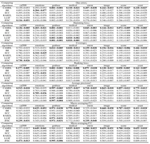
Table 2: Predictive performance of each algorithm (mean±std. deviation) on the regular-scale datasets.

Comparing algorithms

One-error↓

cal500 emotions genbase medical enron image scene yeast

CAMEL 0.129±0.053 0.292±0.052 0.001±0.001 0.110±0.021 0.207±0.038 0.242±0.033 0.175±0.027 0.218±0.027 BR 0.893±0.038 0.284±0.077 0.017±0.016 0.322±0.055 0.646±0.023 0.387±0.027 0.361±0.036 0.244±0.028 ECC 0.295±0.036 0.296±0.074 0.010±0.013 0.156±0.037 0.421±0.034 0.406±0.023 0.306±0.020 0.238±0.030 RAKEL 0.634±0.039 0.300±0.070 0.009±0.007 0.243±0.055 0.532±0.007 0.402±0.024 0.280±0.031 0.244±0.027 LLSF 0.138±0.050 0.412±0.051 0.002±0.005 0.120±0.020 0.250±0.042 0.327±0.030 0.259±0.020 0.394±0.029 JFSC 0.116±0.051 0.438±0.086 0.002±0.005 0.128±0.024 0.278±0.041 0.346±0.023 0.266±0.022 0.242±0.021 Comparing

algorithms

Hamming loss↓

algorithms

Coverage↓

algorithms

Ranking loss↓

algorithms

Average precision↑

algorithms

Macro-averaging F1↑

algorithms

Micro-averaging F1↑

CAMEL 0.337±0.017 0.649±0.041 0.988±0.012 0.835±0.019 0.580±0.023 0.659±0.031 0.780±0.026 0.655±0.010 BR 0.339±0.016 0.639±0.050 0.978±0.014 0.611±0.032 0.359±0.015 0.558±0.028 0.619±0.023 0.633±0.013 ECC 0.364±0.015 0.642±0.046 0.907±0.035 0.796±0.023 0.452±0.015 0.541±0.030 0.653±0.023 0.643±0.017 RAKEL 0.351±0.018 0.629±0.049 0.983±0.011 0.678±0.042 0.392±0.014 0.541±0.031 0.629±0.026 0.632±0.016 LLSF 0.325±0.015 0.637±0.049 0.992±0.003 0.823±0.027 0.534±0.025 0.557±0.032 0.618±0.008 0.280±0.018 JFSC 0.473±0.013 0.406±0.022 0.995±0.006 0.818±0.018 0.555±0.026 0.565±0.033 0.695±0.022 0.609±0.012

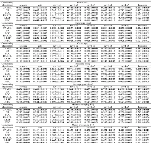
cases, and on the large-scale datasets (Table 3), across all the evaluation metrics, CAMEL ranks first in 69.6% (39/56) cases. Compared with the three well-established algorithms BR, ECC, and RAKEL, CAMEL introduces a new type of label correlations, i.e., collaborative relationships among la-bels, and achieves superior performance in 93.8% (315/336) cases. Compared with the two state-of-the-art algorithms LLSF and JFSC, instead of employing simple similarity measures to regularize the hypothesis space, CAMEL intro-duces a novel method to learn label correlations for explic-itly correlating the final predictions, and achieves superior

performance in 80.4% (180/224) cases. These comparative results clearly demonstrate the effectiveness of the collabo-ration based multi-label learning approach.

(6)

Table 3: Predictive performance of each algorithm (mean±std. deviation) on the large-scale datasets.

Comparing algorithms

One-error↓

science arts rcv1-s1 rcv1-s2 rcv1-s3 rcv1-s4 rcv1-s5 business

algorithms

Hamming loss↓

algorithms

Coverage↓

algorithms

Ranking loss↓

algorithms

Average precision↑

algorithms

Macro-averaging F1↑

algorithms

Micro-averaging F1↑

CAMEL 0.428±0.018 0.415±0.015 0.401±0.015 0.437±0.017 0.431±0.025 0.491±0.017 0.441±0.015 0.746±0.011 BR 0.277±0.013 0.349±0.018 0.301±0.009 0.310±0.009 0.307±0.013 0.356±0.009 0.321±0.009 0.595±0.003 ECC 0.343±0.028 0.377±0.018 0.385±0.016 0.410±0.022 0.414±0.013 0.482±0.024 0.440±0.011 0.690±0.007 RAKEL 0.337±0.014 0.368±0.017 0.341±0.010 0.337±0.008 0.335±0.014 0.369±0.008 0.350±0.008 0.701±0.014 LLSF 0.446±0.025 0.368±0.018 0.463±0.016 0.432±0.018 0.428±0.023 0.478±0.017 0.438±0.019 0.693±0.035 JFSC 0.449±0.026 0.442±0.017 0.456±0.008 0.422±0.011 0.424±0.012 0.482±0.013 0.438±0.011 0.712±0.021

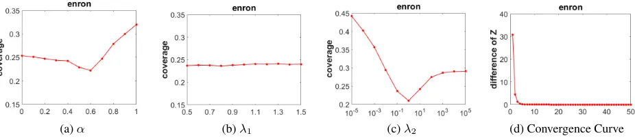
their best setting. Figure 1(a), 1(b), and 1(c) show the sensi-tivity curve of CAMEL with respect toα,λ1, andλ2 respec-tively. It can be seen thatαandλ2have an important influ-ence on the final performance, becauseαandλ2control the collaboration degree and the model complexity. Figure 1(d) illustrates the convergence of CAMEL by using the differ-ence of the optimization variableZbetween two successive iterations, i.e.,∆Z=Z(t)−Z(t−1)_F. From Figure 1(d),

we can observe that∆Zquickly decreases to 0 within a few number of iterations. Hence the convergence of CAMEL is demonstrated.

Conclusion

(7)

simul-(a)α (b)λ1 (c)λ2 (d) Convergence Curve Figure 1: Parameter sensitivity and convergence analysis of CAMEL on the enron dataset.

taneously. Extensive experimental results show that our ap-proach outperforms the state-of-the-art counterparts.

Despite the demonstrated effectiveness of CAMEL, it only considers the global collaborative relationships be-tween labels, by assuming that such collaborative relation-ships are shared by all the instances. However, as different instances have different characteristics, such collaborative relationships may be shared by only a subset of instances rather than all the instances. Therefore, our further work is to explore different collaborative relationships between la-bels for different subsets of instances.

Acknowledgements

This work was supported by MOE, NRF, and NTU.

Appendix A. The ADMM Procedure

To solve problem (3) by ADMM, we first reformulate prob-lem (3) into the following equivalent form:

min

Sj,z 1

2kY−jSi−Yjk 2

2+λkzk1 (13)

s.t. Sj−z= 0

Following the ADMM procedure, the above constrained op-timization problem (13) can be solved as a series of un-constrained minimization problems using augmented La-grangian function, which is presented as:

L(Sj,z,µ) = 1

2kY−jSj−Yjk 2

2+λkzk1+ (14)

v>(Sj−z) +

ρ

2kSj−zk 2 2

Here,ρis the penalty parameter andvis the Lagrange mul-tiplier. By introducing the scaled dual variableµ = 1_ρv, a sequential minimization of the scaled ADMM iterations can be conducted by updating the three variablesSj,zandµ sequentially:

S(k+1)_j = (Y>₋_jY−j+ρI)−1(Y>−jYj+ρ(z(k)−µ(k)))

z(k+1)=Sλ/ρ(S (k+1)

j +µ

(k)₎

µ(k+1)=µ(k)+S(k+1)−z(k+1) (15)

whereSis the proximity operator of the`1norm, which is defined asSω(a) = (a−ω)+−(−a−ω)+.

Appendix B. Model Parameter Optimization

The Lagrangian of problem (8) is expressed as:

L(W,E,A,b) = tr(E>E) +λ2tr(W>W)+ (16)

tr (A>(Z−φ(X)W−1b>−E))

wheretris the trace operator, andA= [a1,a2,· · · ,an]>∈

Rn×q is the introduced matrix that stores the Lagrangian

multipliers. Besides, we have used the property of trace op-erator thattr(W>W) = kWk2_F. By Setting the gradient w.r.t.E,A,W,bto 0 respectively, the following equations will be induced:

∂L

∂E = 0⇒A=E

∂L

∂A = 0⇒Z−φ(X)W−1b

> ₌_E

∂L

∂W = 0⇒W=

1

λ2

φ(X)>A

∂L

∂b = 0⇒A

>₁₌₀ ₍₁₇₎

The above linear equations can be simplified by the follow-ing steps:

Z=φ(X)W+1b>+E

Z= 1

λ2

φ(X)φ(X)>A+1b>+A

Z= 1

λ2

KA+1b>+A (18)

Here, we defineH=_λ1

2K+I, then we can obtain:

HA+1b> =Z

A+H−11b> =H−1Z

1>H−11b> =1>H−1Z

b> = 1H −1_Z

1>_H−1₁ (19)

In this way,Acan be calculated byA=H−1₍_Z₋_1b>₎_.

References

(8)

Boyd, S.; Parikh, N.; Chu, E.; Peleato, B.; Eckstein, J.; et al. 2011. Distributed optimization and statistical learning via the alternating direction method of multipliers.Foundations and TrendsR in Machine learning3(1):1–122.

Cai, X.; Nie, F.; Cai, W.; and Huang, H. 2013. New graph structured sparsity model for multi-label image annotations. In Proceedings of the IEEE International Conference on Computer Vision, 801–808.

Cesa-Bianchi, N.; Gentile, C.; and Zaniboni, L. 2006. Hier-archical classification: combining bayes with svm. In Pro-ceedings of the 23rd International Conference on Machine learning, 177–184.

Elisseeff, A., and Weston, J. 2002. A kernel method for multi-labelled classification. InAdvances in Neural Infor-mation Processing Systems, 681–687.

Gibaja, E., and Ventura, S. 2015. A tutorial on multilabel learning.ACM Computing Surveys47(3):52.

Gopal, S., and Yang, Y. 2010. Multilabel classification with meta-level features. InProceedings of the 33rd international ACM SIGIR Conference on Research and Development in Information Retrieval, 315–322.

Gorski, J.; Pfeuffer, F.; and Klamroth, K. 2007. Biconvex sets and optimization with biconvex functions: A survey and extensions. Mathematical Methods of Operations Research 66(3):373–407.

Hariharan, B.; Zelnik-Manor, L.; Varma, M.; and Vish-wanathan, S. 2010. Large scale max-margin multi-label classification with priors. InProceedings of the 27th Inter-national Conference on Machine Learning, 423–430. Huang, J.; Li, G.; Huang, Q.; and Wu, X. 2016. Learning label-specific features and class-dependent labels for multi-label classification. IEEE Transactions on Knowledge and Data Engineering28(12):3309–3323.

Huang, J.; Li, G.; Huang, Q.; and Wu, X. 2018. Joint feature selection and classification for multilabel learning. IEEE Transactions on Cybernetics48(3):876–889.

Huang, S.-J.; Yu, Y.; and Zhou, Z.-H. 2012. Multi-label hy-pothesis reuse. InProceedings of the 18th ACM SIGKDD In-ternational Conference on Knowledge Discovery and Data Mining, 525–533.

Huang, S.-J.; Zhou, Z.-H.; and Zhou, Z. 2012. Multi-label learning by exploiting label correlations locally. In Proceed-ings of the 26th AAAI Conference on Artificial Intelligence, 949–955.

Ji, S.; Tang, L.; Yu, S.; and Ye, J. 2008. Extracting shared subspace for multi-label classification. InProceedings of the 14th ACM SIGKDD International Conference on Knowl-edge Discovery and Data Mining, 381–389.

Li, X.; Ouyang, J.; and Zhou, X. 2015. Supervised topic models for multi-label classification.Neurocomputing 149:811–819.

Petterson, J., and Caetano, T. S. 2011. Submodular multi-label learning. InAdvances in Neural Information Process-ing Systems, 1512–1520.

Read, J.; Pfahringer, B.; Holmes, G.; and Frank, E. 2011.

Classifier chains for multi-label classification. Machine Learning85(3):333.

Tsoumakas, G.; Dimou, A.; Spyromitros, E.; Mezaris, V.; Kompatsiaris, I.; and Vlahavas, I. 2009. Correlation-based pruning of stacked binary relevance models for multi-label learning. InProceedings of the 1st International Workshop on Learning from Multi-Label Data, 101–116.

Tsoumakas, G.; Spyromitros-Xioufis, E.; Vilcek, J.; and Vlahavas, I. 2011. Mulan: A java library for multi-label learning. Journal of Machine Learning Research 12(7):2411–2414.

Tsoumakas, G.; Katakis, I.; and Vlahavas, I. 2011. Random k-labelsets for multilabel classification. IEEE Transactions on Knowledge and Data Engineering23(7):1079–1089. Yang, H.; Tianyi Zhou, J.; Zhang, Y.; Gao, B.-B.; Wu, J.; and Cai, J. 2016. Exploit bounding box annotations for multi-label object recognition. InProceedings of the IEEE Conference on Computer Vision and Pattern Recognition, 280–288.

Zhang, M.-L., and Zhou, Z.-H. 2006. Multilabel neural networks with applications to functional genomics and text categorization. IEEE Transactions on Knowledge and Data Engineering18(10):1338–1351.

Zhang, M.-L., and Zhou, Z.-H. 2014. A review on multi-label learning algorithms.IEEE Transactions on Knowledge and Data Engineering26(8):1819–1837.

Zhu, S.; Ji, X.; Xu, W.; and Gong, Y. 2005. Multi-labelled classification using maximum entropy method. In Proceed-ings of the 28th International ACM SIGIR Conference on Research and Development in Information Retrieval, 274– 281.