FALSE DYNAMIC EIV MODEL IDENTIFICATION IN THE PRESENCE OF NON-PARAMETRIC DYNAMIC UNCERTAINTY

(1)

Volume 3, Issue 5, May 2014

Page 224

Abstract

For the past decade noise corrupted output measurements have been a fundamental research problem to be investigated. On the other hand, the estimation of the parameters for linear dynamic systems when also the input is affected by noise is recognized as more difficult problem which only recently has received increasing attention. Representations where errors or measurement noises/disturbances are present on both the inputs and outputs are usually called errors-in-variables (EIV) models. In these systems the input is corrupted by noise during measurement only but there is possibility that the noise affects the input and can also affect the output measurements, consequently this gives rise to a false EIV problem [17]. Parameter estimation of this false EIV problem with additive uncertainty effects, with the possibility of noise bearing different assumptions, will be considered in this paper using equation error and output error schemes. The comparative study of these two schemes has also been carried out.

Keywords: Errors-in-variable(EIV), False EIV, additive uncertainty, equation error, output error, Gaussian noise.

1.1 Introduction

In the basic dynamic EIV models the input is corrupted by noise during measurement only but there may be possibility that noise gets added in the input and affects the performance of the system, which can be termed as false EIV problem

[10, 17]. With reference to these systems, the assumptions (prejudices) which lie behind the identification procedure have

been thoroughly analyzed in Kalman with particular attention to the Frisch scheme [7, 9, 10]. This scheme assumes that each variable is affected by an unknown amount of additive noise and each noise component is independent of every other noise component and of every variable. Some classical work on EIV include the work by Adcock, Koopmans (4a), Reiersøl and others whose extensive analysis is given in Anderson [1, 2, 3, 13]. Other works deal with ‘EIV filtering’. This refers to filtering problems, where both input and output measurements are contaminated by noise which has been treated by Guidorzi, Diversi, and Soverini and Markovsky, Willems, and De Moor [8, 12]. Scaled prediction variances in the errors-in-variables models are investigated and their performance is compared with those in classical model of response surface designs [21]. A number of common methods for errors-in-variables methods can be put into a general framework, resulting into a Generalized Instrumental Variable Estimator (GIVE). Söderström presented various computational aspects of GIVE and the asymptotic distribution of the parameter estimates [18].

This paper will be concentrated on the estimation of parameters of false EIV model, with and without additive uncertainty using equation error (EQ) and output error (OP) identification methods [15, 16, 19, 20].

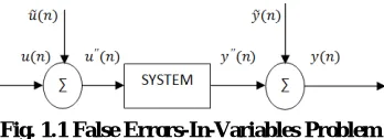
1.2 False dynamic errors-in-variables problem

Dealing with false dynamic EIV models the output measurement noise is considered as a form of process

disturbance and the total effect of and output measurement noise can be modeled as a single auto-correlated

disturbance on the output side as shown in fig. 1.1.

Fig. 1.1 False Errors-In-Variables Problem

Here is the designed input but is added (due to distortions or other unavoidable reasons) before the input reach

the system as which is the noise free input in EIV model. Assumptions on input and output noises can be taken as:

Assumption 1 (A1): When both input and output noises are ARMA (auto regressive moving average) models. Assumption 2 (A2): When input noise is white noise sequence and output noise is ARMA model.

Assumption 3 (A3): When both input and output noises are white noise sequence.

Apart from above assumptions another possibility can be there regarding the noise which may be called as assumption A4.

FALSE DYNAMIC EIV MODEL

IDENTIFICATION IN THE PRESENCE OF

NON-PARAMETRIC DYNAMIC

UNCERTAINTY

Dr (Mrs) Dalvinder Mangal, Dr (Mrs) Lillie Dewan

(2)

Volume 3, Issue 5, May 2014

Page 225

Assumption 4 (A4): When input noise is ARMA model and output noise is white noise sequence.

1.3 False v/s basic dynamic EIV model

 The dynamics between and is the same as between and as shown in Fig. 1.1. Hence the

presence of is not so problematic here as was in basic dynamic EIV model [17].

 affects also the output measurements in case of false dynamic EIV problem.

 For the situation as shown in fig. 1.1, it is appropriate to regard as a form of process disturbance. The total

effect of and can be modeled as a single auto correlated disturbance on the output side.

From the above considered facts it has been realized that false EIV problem is not actually an EIV problem. Therefore the false EIV problem may lie in the following two categories:

Category-1 When both input-output observations are corrupted by noise. Category-2 When only the output observation is corrupted by noise.

In the paper, the false EIV problem with and without additive uncertainty for the category-1 will be identified using EQ and OP formulation for all the assumptions pertaining to input-output noise [4].

1.4 Mathematical formulation for category-1 false EIV model

In this formulation both input-output observations are corrupted by noise and the available signals take the form as: (1.1)

The ARMAX system is given by

(1.2) where

(1.3) Prediction of the output Eq. 1.3 using Eq. 1.2 is given by:

or

(1.4)

(1.5) is the regressor vector

(1.6) is the estimated parameter vector.

The identification of parameters of above described false EIV model will now be carried out considering category-1 with

and without uncertainty for all the four assumptions using EQ and OP formulations [14].

1.5 Case study-I (without uncertainty)

False dynamic errors-in-variables problem is now implemented on the ARX model given as [14]:

(1.7)

where and

and is the nominal model.

The output in periodic form is taken as:

(1.8)

This false EIV model given by Eq. 1.7 is subjected to input-output noise form taken as:

(1.9)

where is the white Gaussian noise with variance 0.01, and is also the white noise with variance 1. is a

random variable and its distribution is uniform within (0, 1). The transfer function of the input-output noise is given by:

(1.10)

(1.11)

In difference equation form:

(3)

Volume 3, Issue 5, May 2014

Page 226

The parameters of false EIV model without uncertainty are estimated using EQ and OP formulations [19] considering all the assumptions A1 to A4.

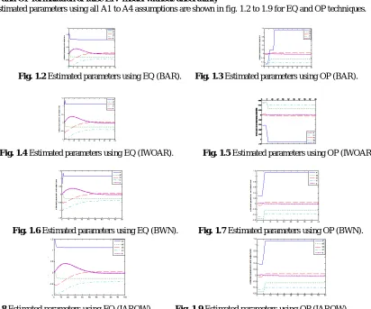
 EQ and OP formulation of false EIV model without uncertainty

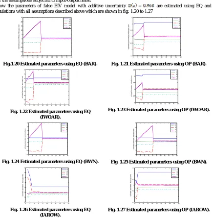
The estimated parameters using all A1 to A4 assumptions are shown in fig. 1.2 to 1.9 for EQ and OP techniques.

Fig. 1.2 Estimated parameters using EQ (BAR). Fig. 1.3 Estimated parameters using OP (BAR).

Fig. 1.4 Estimated parameters using EQ (IWOAR). Fig. 1.5 Estimated parameters using OP (IWOAR).

Fig. 1.6 Estimated parameters using EQ (BWN). Fig. 1.7 Estimated parameters using OP (BWN).

Fig. 1.8 Estimated parameters using EQ (IAROW). Fig. 1.9 Estimated parameters using OP (IAROW).

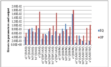
Based on the results from fig. 1.2 to 1.9 the estimated values of the parameters are quantitatively shown using all the four assumptions in table 1.1 for EQ and OP schemes whereas the errors in the parameters and system output are graphically shown by fig.1.10 for these schemes and it has been observed that these errors are very small. Proceeding to this, the assumption wise comparisons for errors in parameters and system output for EQ and OP schemes are given.

Table 1.1 Estimated values of the parameters for false dynamic EIV model using EQ and OP formulation.

True value EQ

(BAR) OP (BAR)

EQ (IWOAR)

OP (IWOAR)

EQ (BWN)

OP (BWN)

EQ (IAROW)

OP (IAROW)

a1 1.131

4

1.1273 1.1376 1.1346 1.1371 1.1360 1.1372 1.1325 1.1363

a2 -0.25 -0.2579 -0.2584 -0.2556 -0.2450 -0.2584 -0.2429 -0.2452 -0.2470

b0 0.05 0.0587 0.0569 0.0570 0.0586 0.0609 0.0580 0.0520 0.0548

(4)

Volume 3, Issue 5, May 2014

Page 227

Fig. 1.10 Errors in true and estimated values of false dynamic EIV model using EQ and OP formulation.

 Comparison of EQ and OP schemes without uncertainty for errors in the parameters and output

 For both input and output noise as ARMA models

- a1⁼ is less for EQ as compared to the a1⁼ of OP scheme.

- b0⁼ is less for OP as compared to the b0⁼ of EQ scheme.

- b1⁼ is less for EQ scheme as compared to the b1⁼ of OP scheme.

- e⁼ is less for EQ as compared to the e⁼ of the OP scheme.

 For input noise as white noise sequence and output noise as ARMA model

- a2⁼ is less for OP as compared to the a2⁼ of EQ scheme.

- b0⁼ is less for EQ as compared to the b0⁼ of OP scheme.

- e⁼ is less for EQ as compared to the e⁼ of the OP schemes.

 For both input and output noise as white noise sequences

- b0⁼ is less for OP as compared to the b0⁼ of EQ scheme.

 For input noise as ARMA model and output noise as white noise sequence

- b0⁼ is less for EQ as compared to the b0⁼ of OP scheme.

After analyzing the results obtained above it is concluded that when false EIV model without uncertainty is identified by using equation error and output error formulation considering the category-1 (both input-output observations corrupted by measurement noise) the equation error formulation is giving less error in almost all the parameters and hence output as compared to output error scheme in all the possibilities of noise entering into the system.

1.6 Case study-II (with uncertainty)

The parameters of the system given by Eq. 1.7 are estimated considering all the four assumptions A1-A4 pertaining to input-output noise using EQ and OP methods [19]. The ARMA model of the input-output noise is given by Eq. 1.12 and 1.13 respectively whose general form is given by Eq. 1.9. The input to the system is periodic given by Eq. 1.8. The system is perturbed by additive uncertainty given by Eq. 1.14 and 1.15 respectively [15]:

(1.14)

where is the perturbed plant.

and (1.15)

where is the perturbation bound based on a priori physical information.

Here the two cases for the additive uncertainty have been considered [5, 6, 20]:

(5)

Volume 3, Issue 5, May 2014

Page 228

The parameters of false EIV model with additive uncertainty and are estimated using EQ and OP

formulations considering all the assumptions A1 to A4.

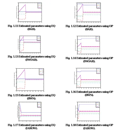
The estimated parameters using all the assumptions are shown in fig. 1.11 to 1.18 for EQ and OP formulations with .

 The estimated parameters using all the assumptions are shown in fig. 1.11 to 1.18 for EQ and OP formulations

with .

Table 1.2 Estimated values of the parameters for false dynamic EIV model using EQ and OP formulation with .

0 5 10 15 20 25 30 35 40 45 50 -15 -10 -5 0 5 10 15 e s ti m a te d p a ra m e te rs a n d o u tp u t e rr o r a1 a2 b0 b1 e

Fig. 1.11 Estimated parameters using EQ (BAR).

0 5 10 15 20 25 30 35 40 45 50 -1.5 -1 -0.5 0 0.5 1 1.5 e s ti m a te d p a ra m e te rs a n d o u tp u t e rr o r a1 a2 b0 b1 e

Fig. 1.12 Estimated parameters using OP (BAR).

0 5 10 15 20 25 30 35 40 45 50 -5 -4 -3 -2 -1 0 1 2 3 es tim at ed param et er s and out pu t error a1 a2 b0 b1 e

Fig. 1.13 Estimated parameters using EQ (IWOAR).

0 5 10 15 20 25 30 35 40 45 50 -1 -0.5 0 0.5 1 1.5 e s ti m a te d p a ra m e te rs a nd o u tp u t e rr o r a1 a2 b0 b1 e

Fig. 1.14 Estimated parameters using OP (IWOAR).

0 5 10 15 20 25 30 35 40 45 50 -15 -10 -5 0 5 10 15 e s ti m a te d p a ra m e te rs a n d o u tp u t e rr o r a1 a2 b0 b1 e

Fig. 1.15 Estimated parameters using EQ (BWN).

0 5 10 15 20 25 30 35 40 45 50 -1 -0.5 0 0.5 1 1.5 e s ti m a te d p a ra m e te rs a n d o u tp u t e rr o r a1 a2 b0 b1 e

Fig. 1.16 Estimated parameters using OP (BWN).

0 5 10 15 20 25 30 -2 -1 0 1 2 3 4 5 e s ti m a te d p a ra m e te rs a n d o u tp u t e rr o r a1 a2 b0 b1 e

Fig. 1.17 Estimated parameters using EQ (IAROW).

0 5 10 15 20 25 30 35 40 45 50 -1.5 -1 -0.5 0 0.5 1 1.5 e s ti m a te d p a ra m e te rs a n d o u tp u t err o r a1 a2 b0 b1 e

Fig. 1.18 Estimated parameters using OP (IAROW).

True value EQ

(BAR) OP (BAR) EQ (IWOAR) OP (IWOAR) EQ (BWN) OP (BWN) EQ (IAROW) OP (IAROW)

a1 1.1314 1.1516 1.1338 1.1375 1.1334 1.1414 1.1339 1.269 1.1332

a2 -0.25 -0.2580 -0.2519 -0.2575 -0.2518 -0.2549 -0.2522 -0.2456 -0.2489

b0 0.05 0.0588 0.0526 0.0594 0.0519 0.0600 0.0526 0.0563 0.0513

(6)

Volume 3, Issue 5, May 2014

Page 229

Fig. 1.19 Errors in true and estimated values of false dynamic EIV model using EQ and OP formulation with .

 Comparison of EQ and OP schemes with for errors in the parameters and output

- The error in the parameters and system output is minimum for output error algorithm as compared to equation error for

all the assumptions subjected to input-output noise.

Now the parameters of false EIV model with additive uncertainty are estimated using EQ and OP

formulations with all assumptions described above which are shown in fig. 1.20 to 1.27

0 5 10 15 20 25 30 35 40 45 50 -20 -15 -10 -5 0 5 10 15 20 25 e s ti m a te d p a ra m e te rs a n d o u tp u t e rr o r a1 a2 b0 b1 e

Fig.1.20 Estimated parameters using EQ (BAR).

Fig. 1.21 Estimated parameters using OP (BAR).

0 5 10 15 20 25 30 35 40 45 50 -5 -4 -3 -2 -1 0 1 2 3 e s ti m a te d p a ra m e te rs a n d o u tp u t e rr o r a1 a2 b0 b1 e

Fig. 1.22 Estimated parameters using EQ (IWOAR).

0 5 10 15 20 25 30 35 40 45 50 -1 -0.5 0 0.5 1 1.5 e s ti m a te d p a ra m e te rs a n d o u tp u t e rr o r a1 a2 b0 b1 e

Fig. 1.23 Estimated parameters using OP (IWOAR).

0 5 10 15 20 25 30 35 40 45 50 -20 -15 -10 -5 0 5 10 15 20 e s ti m ate d p a ra m e te rs a n d o u tp u t e rr o r a1 a2 b0 b1 e

Fig. 1.24 Estimated parameters using EQ (BWN).

0 5 10 15 20 25 30 35 40 45 50 -6 -4 -2 0 2 4 6 8 e s ti m a te d p a ra m e te rs a n d o u tp u t e rr o r a1 a2 b0 b1 e

Fig. 1.25 Estimated parameters using OP (BWN).

0 2 4 6 8 10 12 14 16 18 20 -2 -1 0 1 2 3 4 5 e s ti m a te d p a ra m e te rs a n d o u tp u t e rr o r a1 a2 b0 b1 e

Fig. 1.26 Estimated parameters using EQ (IAROW).

(7)

Volume 3, Issue 5, May 2014

Page 230

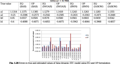
Based on the results from fig. 1.20 to 1.27 the estimated values of the parameters are quantitatively shown using all the four assumptions in table 1.3 for EQ and OP schemes whereas the errors in the parameters and system output are graphically shown in fig.1.28 for these schemes and it has been observed that these errors are very small.

Table 1.3 Estimated values of the parameters for false dynamic EIV model using EQ and OP formulation

with .

True value EQ

(BAR) OP (BAR)

EQ (IWOAR)

OP (IWOAR)

EQ (BWN)

OP (BWN)

EQ (IAROW)

OP (IAROW)

a1 1.1314 1.1375 1.1385 1.1279 1.1418 1.1243 1.1263 1.1283 1.1355

a2 -0.25 -0.2586 -0.2573 -0.2542 -0.2585 -0.2431 -0.2563 -0.2471 -0.2448

b0 0.05 0.0557 0.0581 0.0578 0.0560 0.0561 0.0603 0.0459 0.0542

b1 -0.4 -0.4088 -0.4071 -0.4055 -0.4075 -0.3943 -0.4064 -0.3968 -0.4057

Fig. 1.28 Errors in true and estimated values of false dynamic EIV model using EQ and OP formulation

with .

From the above table it is clear that the error in parameters and hence output is less using equation error formulation as compared to output error algorithm for all the assumptions subjected to input-output noise.

1.7 Conclusion

From the analysis of the results obtained above it is concluded that when false EIV model without uncertainty is identified by using equation error and output error formulation considering both input-output observations corrupted by measurement noise, the equation error formulation is giving less error in almost all the parameters as compared to output error scheme for all the assumptions subjected to input-output noise. When the same model is identified for

using equation error and output error algorithms considering then it is found that the error in all the parameters and output is minimum for output error as compared to equation error. On the other hand when this case is considered for it is found that the error in parameters and hence output is less using equation error formulation as compared to output error algorithm.

REFERENCES

[1] Adcock, R. J., “ Note on the methods of least squares”, The Analyst, 4(6), pp. 183–184, 1877.

[2] Adcock, R. J., “ A problem in least squares”, The Analyst, 5(2), pp. 53–54, 1878.

[3] Anderson, B. D. O., & Deistler, M., “Identifiability of dynamic errorsin- variables models”, Journal of Time Series

Analysis, 5, pp. 1–13, 1984.

[4] Bombois, X., Gevers, M., Scorletti, G., Anderson, B. D. O., “Robustness analysis tools for an uncertainty set obtained

by prediction error identification”, Automatica, 37, pp. 1629-1636, 2001.

[5] Douma, S. G., Paul M.J., Van den Hof, Bosgra, O. H., “Controller tuning freedom under plant identification

uncertainty: double Youla beats gap in robust stability”, Proceedings of the American Control Conference, Arlington,

June, pp. 3153-3158, 2001.

[6] Douma, S. G., Van den Hof, Paul. M. J., Bosgra, O. H., “Controller tuning freedom under plant identification

uncertainty: double Youla beats gap in robust stability”, Automatica, 39(2), pp. 325-333, 2003.

[7] Frisch, R., “Statistical confluence analysis by means of complete regression systems”, Technical Report 5, University

of Oslo, Economics Institute, Oslo, Norway. 1934.

(8)

Volume 3, Issue 5, May 2014

Page 231

[9] Kalman, R. E., “Identification from real data”, In: M. Hazewinkel, & A. H. G. Rinnoy Kan (Eds.), Current

developments in the interface: Economics, econometrics, mathematicsDordrecht, The Netherlands: Reidel. 1982a.

[10]Kalman, R. E., “System identification from noisy data”, In: Bednarek, A.R., Cesari, L., (Eds.),“Dynamical systems II”

New York, NY: Academic Press. 1982b.

[11]Koopmans, T. J., “Linear regression analysis of economic time series”, The Netherlands: N. V. Haarlem, 1937.

[12]Markovsky, I., Willems, J. C., & De Moor, B., “Continuous-time errors-in-variables filtering”, In 41st conference on

decision and control (CDC 2002), Las Vegas, Nevada, pp. 2576–2581, December 2002.

[13]Reiersøl, O., “Identifiability of a linear relation between variables which are subject to error”, Econometrica, 18(4),

pp. 375–389, 1950.

[14]Shynk, J.J., “Adaptive IIR Filtering”, IEEE ASSP Magazine, April, 4-21, 1989.

[15]Sippe G. Douma, Paul M.J., Van den Hof, “Relations between uncertainty structures in identification for robust

control”, Automatica, 41, pp. 439-457, 2005.

[16]Söderström, T., Soverini, U., Mahata, K., “Perspectives on errors-in-variables estimation for dynamic systems”, Signal

Processing, 82(8), pp. 1139-1154, 2002.

[17]Söderström, T., “Errors-in-variables methods in system identification”, Automatica, 43, pp. 939-958, 2007.

[18]Söderström, T., “A generalized instrumental variable estimation method for errors-in- variables identification

problems”. Automatic. 47(8), August, pp. 1656-1666, 2011.

[19]Xianhua, D., Zhenya, H., “Robust Adaptive System Identification By Using Median smoothing”, IEEE Conference,

Southeast University, Nanjing 210018, P.R.China, pp. 564-567, 1991.

[20]Younce R. C., Rohrs C. E., “Identification with non-parametric uncertainty”, Proceedings of the 29th Conference on

decision and control, Honolulu, Hawali, December, pp. 3154-3161, 1990.

[21] Zheng, HE, Fang, J., “Comparative study of response surface designs with errors-in-variables model”, Trans. Tianjin

Univ., 17, pp. 146-150, 2011.

Dr (Mrs) Dalvinder Mangal Born on February 21, 1977 at (Nilokheri) Karnal, Haryana, India, the land of Karna, Ms Dalvinder Kaur Mangal received her B.E. (Hons.), M.E. and Ph.D. degrees from DCRUST, Murthal, P.U. Chandigarh and NIT, Kurukshetra respectively in the field of Electrical Engineering. As a teacher she dedicatedly contributed her services at various colleges and Institutes of Haryana. Presently she is working as an Assistant Professor, Department of Electronics & Instrumentation Engineering, at The Technological Institute of Textile and Sciences, Bhiwani, Haryana, India. She has attended various National and International seminars and conferences. She presented/published several papers in the Journals of International/National repute.

Electronics and Instrumentation Engineering Department, The Technological Institute of Textile and Sciences, Bhiwani (127021), Haryana, India.

Dr (Mrs) Lillie Dewan is a professor. She has numerous research papers in international/national journals and conferences to her credit. Her current research interest areas include identification and robust control, digital signal processing, image processing, and electrical machines. E-mail: