Volume 3 Number 1 2012 pp. 1-15 ISSN: 1309-2448 www.berjournal.com
Co-movements of and Linkages between Asian Stock Markets
Ilhan Meric
aJoe H. Kim
bAbstract: International marketers may be interested in stock market linkages for various reasons: the co-movements of equity prices appear to reflect not only market globalization but also the globalization of capital resources. The co-movements can affect the balancing strategies of country market portfolios as they indicate opportunities and risks. The strategic choice of alternative market presence, such as market entry via export marketing or a full ownership and marketing may need to match with the type of financial resources. The co-movements of and the linkages between the U.S. stock market and Asian stock markets have been studied extensively. However, little attention has been given to the co-movements of Asian stock markets and the lead/lag linkages between them. In this paper, we study this issue with the principal components analysis (PCA) and Granger-causality (G-C) statistical techniques. We find that the contemporaneous co-movements of Asian stock markets have become closer and portfolio diversification benefits with Asian stock markets have diminished over time during the January 1, 2001-January 1, 2011 period. We find that the Singapore, Indian, and Japanese stock markets are the most influential stock markets and the Philippine and South Korean stock markets are the least influential stock markets in Asia. The Japanese, Singapore, and New Zealand stock markets are the least affected stock markets and the Shanghai, Australian, and South Korean stock markets are the most affected stock markets by the movements in the other Asian stock markets.
Keywords: Asian stock markets, Co-movements of stock markets, Linkages between stock markets, Principal components analysis, Granger causality
JEL Classification:G11, G15
1. Introduction
In this paper, we study the contemporaneous co-movements of Asian stock markets and the time series lead/lag linkages between them with the principal components analysis (PCA) and Granger causality (G-C) statistical techniques with a sample of thirteen major Asian stock markets during the January 1, 2001-January 1, 2011 period.
Studying the contemporaneous co-movements of national stock markets has long been a popular research topic in finance (see: Meric and Meric, 2011). Makridakis and Wheelwright (1974), Philippatos, Christofi, and Christofi (1983), and Meric and Meric (1989) have made the use of the PCA multivariate technique popular in studying the co-movements of national stock markets. The technique has since been used in many studies (see, eg., Lee and Kim, 1993; Lau and McInnish, 1993; Meric and Meric, 1996, 1997, 2001a,b). In this paper, we use the PCA techniques to study the contemporaneous co-movement patterns of Asian stock markets with daily index returns data for the January 1, 2001-January 1, 2011 period.
We divide the 10-year period into two 5-year sub-periods and we apply PCA to each period to determine if there are significant changes in the co-movement patterns of Asian stock markets over time.
In empirical studies, the G-C technique is often used to determine if the past index returns of a national stock market can be used to predict the future index returns of other national stock markets (see, e.g., Ratner and Leal, 1996; Meric et al., 2002; Meric and Meric, 2011). In this paper, we use the G-C technique to study the lead/lag linkages between Asian stock markets with daily stock market index data for the January 1, 2001-January 1, 2011 period. We determine the most influential and the least influential stock markets in Asia. We investigate which Asian stock markets are leading the others and which Asian stock markets tend to follow the others. We determine the Asian stock markets that are most affected and those that are least affected by the movements of the other Asian stock markets.
The paper is organized as follows. In the next section, we explain our data and methodology. We present our PCA results in Section III. We present our G-C analysis results in Section IV. We summarize our findings and present our conclusions in Section V. We describe the PCA and G-C statistical techniques in Appendixes A and B, respectively.
2. Data and Methodology
The study covers the following thirteen Asian stock markets: Australia, Hong Kong, India, Indonesia, Japan, Malaysia, New Zealand, the Philippines, Singapore, Shanghai, South Korea, Taiwan, and Thailand. The daily stock market indexes for these stock markets were downloaded from the DataStream database. The Morgan Stanley Capital International (MSCI) data are used for the Indonesian and South Korean stock markets. The DataStream data are used for the other stock markets. The daily stock returns were computed as the log difference in the indexes (Ln(It/It-1)).
The principal component analysis (PCA) is a widely used multivariate statistical technique to study the contemporaneous co-movements of global equity markets. The PCA technique can combine global stock markets into distinct principal component clusters in terms of the similarities of their contemporaneous co-movements. Stock markets with correlated, close co-movement patterns are not good portfolio diversification prospects. We determine which Asian stock markets were good portfolio diversification prospects for investors during the January 1, 2001-January 1, 2011 period. We use the PCA technique to study the contemporaneous co-movement patterns of the Asian stock markets. A brief description of the PCA techniques is presented in Appendix A. A detailed discussion of the technique can be found in Mardia, Kent, and Bibby (1979) and Marascuilo and Levin (1983).
stock markets are leading the other Asian stock markets and which Asian stock markets are affected the most by the movements in the other Asian stock markets. Stock markets with significant lead/lag linkages are not good portfolio diversification prospects for investors.
3. Principal Components Analysis
To determine the clusters of stock markets with similar contemporaneous movement patterns, the correlation matrix of the thirteen Asian stock markets was used as input in the SPSS-PCA program. The Varimax rotation was used to maximize the factor loadings of the stock markets in each principal component with similar movement patterns. Using Kaiser's significance rule, statistically significant principal components with eigenvalues greater than unity were retained for analysis (see: Mardia et al., 1979, Marascuilo and Levin, 1983). The January 1, 2001-January 1, 2011 ten-year period was divided into two five-year sub-periods and the analysis was applied to each sub-period separately.
3.1. January 1, 2001-January 1, 2006 Period
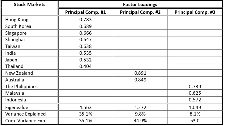
There are three statistically significant principal components for this period. The highest factor loadings for the thirteen stock markets in the three principal components are presented in Table 1. The stock markets with high factor loadings in the same principal component have similar contemporaneous movement patterns and they are highly correlated. Therefore, having these stock markets in the same investment portfolio would provide limited diversification benefits. To maximize the portfolio diversification benefit, investors should invest in the stock markets with high factor loadings in different principal components.
The first principal component is dominated by the Hong Kong, South Korean, Singapore, Shanghai, Taiwanese, Indian, Japanese, and Thai stock markets. This principal component has an eigenvalue of 4.563 and it explains 35.1 percent of the variation in the original data matrix. The New Zealand and Australian stock markets have their highest factor loadings in the second principal component. This principal component has an eigenvalue of 1.272 and it
Table 1. Principal Components Analysis: January 1, 2001-January 1, 2006 Period
Stock Markets Factor Loadings
Principal Comp. #1 Principal Comp. #2 Principal Comp. #3
Hong Kong 0.783
South Korea 0.689
Singapore 0.666
Shanghai 0.647
Taiwan 0.638
India 0.535
Japan 0.532
Thailand 0.404
New Zealand 0.891
Australia 0.849
The Philippines 0.739
Malaysia 0.625
Indonesia 0.572
Eigenvalue 4.563 1.272 1.049
Variance Explained 35.1% 9.8% 8.1%
explains 9.8 percent of the variation in the original data matrix. The Philippine, Malaysian, and Indonesian stock markets have their highest factor loadings in the third principal component. This principal component has an eigenvalue of 1.049 and it explains 8.1 percent of the variation in the original data matrix. All three principal components together can explain 53.0 percent of the variance in the original data matrix.
3.2. January 1, 2006-January 1, 2011 period
The analysis is also applied to the January 1, 2006-January 1, 2011 period to determine if there are any significant changes in the contemporaneous co-movement patterns of Asian stock markets over time. This time period includes the 2008 global stock market crash and the post-crash recovery in 2009, when all global stock markets moved closely together. Therefore, one would expect that the number of statistically significant principal components would decrease and the benefits of global portfolio diversification would diminish during this period.
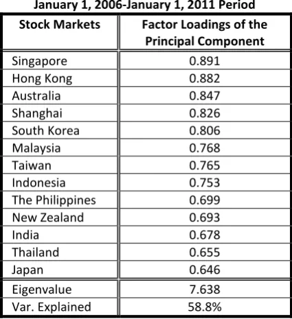
Indeed, there is only one statistically significant principal component for the January 1, 2006-January 1, 2011 period. The factor loadings of the principal component are presented in Table 2. The principal component has an eigenvalue of 7.638 and it explains 58.8 percent of the variation in the original data matrix.
There are three statistically significant principal components in the January 1, 2001-January 1, 2006 period versus only one statistically significant principal component in the January 1, 2006-January 1, 2011 period. This indicates that the co-movements of Asian stock markets became considerably closer and the portfolio diversification benefits of investing in Asian stock markets decreased significantly from the first year period to the second five-year period.
Table 2. Principal Components Analysis: January 1, 2006-January 1, 2011 Period Stock Markets Factor Loadings of the
Principal Component
Singapore 0.891
Hong Kong 0.882
Australia 0.847
Shanghai 0.826
South Korea 0.806
Malaysia 0.768
Taiwan 0.765
Indonesia 0.753
The Philippines 0.699
New Zealand 0.693
India 0.678
Thailand 0.655
Japan 0.646
Eigenvalue 7.638
4. Granger-Causality Tests
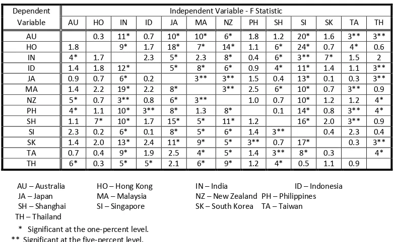
The Estima RATS Granger-Sims computer program was used in the Granger causality (G-C) tests. The optimal lag-length is three trading days in the VAR system used in the analysis (see: Sims, 1980). The G-C test results for the joint hypotheses of zero coefficients on all three lags for each stock market are presented in Table 3.
4.1. General Observations
The stock markets with significant lead/lag linkages are not good portfolio diversification prospects. The findings show that Asian stock markets have significant lead/lag linkages. The F-value statistics in Table 3 indicate that most Asian stock markets have significant influence on the other Asian stock markets (i.e., the past returns of most Asian stock markets can predict the future returns of other Asian stock markets. 65 of the 156 F-value statistics are statistically significant at the one-percent level. 18 test statistics are significant at the five-percent level.
The sum of the F-value statistics in each column of Table 3 shows the influence of each Asian stock market on the other Asian stock markets as an independent variable. The sum is the highest for the Singapore (146.5), Indian (113), and Japanese (98.6) stock markets. These stock markets appear to be the most influential stock markets in Asia. The sum is the lowest for the South Korean (17.3) and Philippine (17.4) stock markets. These stock markets appear to be the least influential stock markets in Asia.
All of the F-value statistics for the Indian stock market as an independent variable are statistically significant (i.e., the past returns of the Indian stock market leads -can predict- the stock returns of all the other Asian stock markets). Except the Thai stock market, the past returns of the Singapore stock market leads (can predict) the future stock returns of all the
Table 3. Granger-Causality Test Statistics: January 1, 2001-January 1, 2011
Dependent Variable
Independent Variable - F Statistic
AU HO IN ID JA MA NZ PH SH SI SK TA TH
AU 0.3 11* 0.7 10* 10* 6* 1.8 1.2 20* 1.6 3** 3** HO 1.8 9* 1.7 18* 7* 14* 1.1 6* 24* 0.7 4* 0.6
IN 4* 1.7 2.3 5* 2.3 8* 0.4 6* 3** 7* 1.5 2
ID 1.4 1.8 12* 5* 8* 6* 0.9 4* 11* 1.4 1.1 3** JA 0.9 0.7 6* 0.2 3** 3** 1.5 0.4 13* 0.1 0.3 3** MA 1.4 2.2 19* 2.2 8* 3** 2.5 6* 10* 0.7 3** 0.9 NZ 5* 0.7 3** 0.8 6* 3** 1.0 0.7 10* 1.2 1.2 4* PH 4* 1.1 10* 3** 8* 1.3 8* 0.1 14* 0.8 3** 4* SH 1.1 7* 10* 1.7 15* 5* 11* 1.2 16* 2.0 3** 0.9 SI 2.3 0.2 6* 0.1 8* 5* 6* 1.4 3** 0.4 2.3 0.4 SK 1.4 2.0 13* 2.4 11* 9* 5* 3** 0.7 17* 0.3 3** TA 0.7 0.4 9* 1.9 2.5 4* 5* 1.4 3** 8* 0.3 4* TH 6* 0.3 5* 5* 2.1 6* 9* 1.2 4* 0.5 1.1 0.9
AU – Australia HO – Hong Kong IN – India ID – Indonesia JA – Japan MA – Malaysia NZ – New Zealand PH – Philippines
SH – Shanghai SI – Singapore SK – South Korea TA – Taiwan TH – Thailand
other Asian stock markets. Except the Thai and Taiwanese stock markets, the past returns of the Japanese stock market lead (can predict) the future stock returns of all the other Asian stock markets. The past returns of the South Korean stock market leads (can predict) the future stock returns of only the Indian stock market. The past returns of the Philippine stock market leads (can predict) the future stock returns of only the South Korean stock market.
The horizontal sum of the F-value statistics in Table 3 shows to what extent each Asian stock market is influenced by the other Asian stock markets as a dependent variable (i.e., to what extend the future returns of an Asian market can be predicted by the past returns of the other Asian stock markets). The sum is the highest for the Shanghai (73.9), Australian (68.6), and South Korean (67.8) stock markets (i.e., these stock markets are the most influenced Asian stock markets by the other Asian stock markets). The sum is the lowest for the Japanese (32.1), Singapore (35.1), and New Zealand (36.6) stock markets (i.e., these stock markets are the least influenced Asian stock markets by the other Asian stock markets).
4.2. Australia
The returns of the Australian stock market lead the returns of the Indian, New Zealand, Philippine, and Thai stock markets (i.e., the past returns of the Australian stock market can predict the future returns of the Indian, New Zealand, Philippine, and Thai stock markets). The F statistics for these stock markets are all significant at the one-percent level.
The returns of the Australian stock market appear to follow the returns of the Indian, Japanese, Malaysian, New Zealand, Singapore, Taiwanese, and Thai stock markets (i.e., the past returns of the Indian, Japanese, Malaysian, New Zealand, Singapore, Taiwanese, and Thai stock markets can predict the future returns of the Australian stock market). The F statistics for the Indian, Japanese, Malaysian, New Zealand, and Singapore stock markets are significant at the one-percent level. The F statistics for the Taiwanese and Thai stock markets are significant at the five-percent level.
4.3. Hong Kong
The returns of the Hong Kong stock market appear to lead only the returns of the Shanghai stock market (i.e., the past returns of the Hong Kong stock market can predict the future returns of only the Shanghai stock market). The F statistic is significant at the one-percent level.
The returns of the Hong Kong stock market appear to follow the returns of the Indian, Japanese, Malaysian, New Zealand, Shanghai, Singapore, and Taiwanese stock markets (i.e., the past returns of the Indian, Japanese, Malaysian, New Zealand, Shanghai, Singapore, and Taiwanese stock markets can predict the future returns of the Hong Kong stock market). All F statistics are significant at the one-percent level.
4.4. India
The returns of the Indian stock market appear to follow the returns of the Australian, Japanese, New Zealand, Shanghai, Singapore, and South Korean stock markets (i.e., the past returns of the Australian, Japanese, New Zealand, Shanghai, Singapore, and South Korean stock markets can predict the future returns of the Indian stock market). The test statistics for the Australian, Japanese, Shanghai, and South Korean stock markets are significant at the one-percent level. The F statistic for the Singapore stock market is significant only at the five-percent level.
4.5. Indonesia
The returns of the Indonesian stock market appear to lead only the returns of the Philippine and Thai stock markets (i.e., the past returns of the Indonesian stock market can predict the future returns of the Philippine and Thai stock market). The test statistic for the Thai stock market is significant at the one-percent level. The test statistic for the Philippine stock market is significant at the five-percent level.
The returns of the Indonesian stock market appear to follow the returns of the Indian, Japanese, Malaysian, New Zealand, Shanghai, Singapore, and Thai stock markets (i.e., the past returns of the Indian, Japanese, Malaysian, New Zealand, Shanghai, Singapore, and Thai stock markets can predict the future returns of the Indonesian stock market). The F statistics for the Indian, Japanese, Malaysian, New Zealand, Shanghai, and Singapore stock markets are significant at the one-percent level. The F statistic for the Thai stock market is significant only at the five-percent level.
4.6. Japan
The returns of the Japanese stock market lead the returns of all the other Asian stock markets except the Taiwanese and Thai stock markets (i.e., the past returns of the Japanese stock market can predict the future returns of all the other Asian stock markets except the Taiwanese and Thai stock markets). The test statistics for the Australian, Hong Kong, India, Indonesian, Malaysian, New Zealand, Philippine, Shanghai, Singapore, and South Korean stock markets are all significant at the one-percent level.
The returns of the Japanese stock market appear to follow the returns of the Indian, Malaysian, New Zealand, Singapore, and Thai stock markets (i.e., the past returns of the Indian, Malaysian, New Zealand, Singapore, and Thai stock markets can predict the future returns of the Japanese stock market). The test statistics for the Indian and Singapore stock markets are significant at the one-percent level. The test statistics for the Malaysian, New Zealand, and Thai stock markets are significant at the five-percent level.
4.7. Malaysia
The returns of the Malaysian stock market appear to follow the returns of the Indian, Japanese, New Zealand, Shanghai, Singapore, and Taiwanese stock markets (i.e., the past returns of the Indian, Japanese, New Zealand, Shanghai, Singapore, and Taiwanese stock markets can predict the future returns of the Malaysian stock market). The test statistics for the Indian, Japanese, Shanghai, and Singapore stock markets are significant at the one-percent level. The test statistics for the New Zealand and Taiwanese stock markets are significant at the five-percent level.
4.8. New Zealand
The returns of the New Zealand stock market appear to lead the returns of all the other Asian stock markets (i.e., the past returns of the New Zealand stock market can predict the future returns of all the other Asian stock markets). The test statistics for the Australian, Hong Kong, Indian, Philippine, Shanghai, Singapore, South Korean, Taiwanese, and Thai stock markets are significant at the one-percent level. The test statistics for the Japanese and Malaysian stock markets are significant at the five-percent level.
The returns of the New Zealand stock market follow the returns of the Australian, Indian, Japanese, Malaysian, Singapore, and Thai stock markets (i.e., the past returns of the Australian, Indian, Japanese, Malaysian, Singapore, and Thai stock markets can predict the future returns of the New Zealand stock market). The test statistics for the Australian, Japanese, Singapore, and Thai stock markets are significant at the one-percent level. The test statistics for the Indian and Malaysian stock markets are significant at the five-percent level.
4.9. The Philippines
The returns of the Philippine stock market appear to lead the returns of only the South Korean stock market (i.e., the past returns of the Philippine stock market can predict the future returns of only the South Korean stock market). The test statistic for the South Korean stock market is significant at the five-percent level.
The returns of the Philippine stock market follow the returns of the Australian, Indian, Indonesian, Japanese, New Zealand, Singapore, Taiwanese, and Thai stock markets (i.e., the past returns of the Australian, Indian, Indonesian, Japanese, New Zealand, Singapore, Taiwanese, and Thai stock markets can predict the future returns of the Philippine stock market). The test statistics for the Australian, Indian, Japanese, New Zealand, and Singapore stock markets are significant at the one-percent level. The test statistics for the Indonesian and Thai stock markets are significant at the five-percent level.
4.10. Shanghai
The returns of the Shanghai stock market appear to follow the returns of the Indian, Japanese, Malaysian, New Zealand, Singapore, Taiwanese, and Thai stock markets (i.e., the past returns of the Indian, Japanese, Malaysian, New Zealand, Singapore, Taiwanese, and Thai stock markets can predict the future returns of the Shanghai stock market). The F statistics for the Indian, Japanese, Malaysian, New Zealand, and Singapore stock markets are significant at the one-percent level. The F statistics for the Taiwanese and Thai stock markets are significant only at the five-percent level.
4.11. Singapore
The returns of the Singapore stock market lead the returns of all the other Asian stock markets except the Thai stock market (i.e., the past returns of the Malaysian stock market can predict the future returns of all the other Asian stock markets except the Thai stock market). The test statistics for the Australian, Hong Kong, Indonesian, Japanese, Malaysian, New Zealand, Philippine, Shanghai, South Korean, and Taiwanese stock markets are significant at the one-percent level. The test statistic for the Indian stock market is significant only at the five-percent level.
The returns of the Singapore stock market appear to follow the returns of the Indian, Japanese, Malaysian, New Zealand, and Shanghai stock markets (i.e., the past returns of the Indian, Japanese, Malaysian, New Zealand, and Shanghai stock markets can predict the future returns of the Singapore stock market). The test statistics for all of these stock markets are significant at the one-percent level.
4.12. South Korea
The returns of the South Korean stock market appear to lead the returns of only the Indian stock market (i.e., the past returns of the South Korean stock market can predict the future returns of only the Indian stock market). The test statistic is significant at the one-percent level.
The returns of the South Korean stock market follow the returns of the Indian, Japanese, Malaysian, New Zealand, Philippine, Singapore, and Thai stock markets (i.e., the past returns of the Indian, Japanese, Malaysian, New Zealand, Philippine, Singapore, and Thai stock markets can predict the future returns of the South Korean stock market). The test statistics for the Indian, Japanese, Malaysian, New Zealand, and Singapore stock markets are significant at the one-percent level. The test statistics for the Philippine and Thai stock markets are significant at the five-percent level.
4.13. Taiwan
The returns of the Taiwanese stock market lead the returns of the Australian, Hong Kong, Malaysian, Philippine, and Shanghai stock markets (i.e., the past returns of the Taiwanese stock market can predict the future returns of the Australian, Hong Kong, Malaysian, Philippine, and Shanghai stock markets). The test statistic for the Hong Kong stock market is significant at the one-percent level. The test statistics for the other stock markets are significant at the five-percent level.
Indian, Malaysian, New Zealand, Shanghai, Singapore, and Thai stock markets can predict the future returns of the Taiwanese stock market). The test statistics for the Indian, Malaysian, New Zealand, Singapore, and Thai stock markets are significant at the one-percent level. The test statistic for the Shanghai stock market is significant only at the five-percent level.
4.14. Thailand
The returns of the Thai stock market lead the returns of the Australian, Indonesian, Japanese, New Zealand, Philippine, South Korean, and Taiwanese stock markets (i.e., the past returns of the Thai stock market can predict the future returns of the Australian, Indonesian, Japanese, New Zealand, Philippine, South Korean, and Taiwanese stock markets). The test statistics for the New Zealand, Philippine, and Taiwanese stock markets are significant at the one-percent level. The test statistics for the Australian, Indonesian, Japanese and South Korean, stock markets are significant at the five-percent level.
The returns of the Thai stock market follow the returns of the Australian, Indonesian, Japanese, New Zealand, Philippine, South Korean, and Taiwanese stock markets (i.e., the past returns of the Australian, Indonesian, Japanese, New Zealand, Philippine, South Korean, and Taiwanese stock markets can predict the future returns of the Thai stock market). The test statistics for the New Zealand, Philippine, and Taiwanese stock markets are significant at the one-percent level. The test statistic for the Australian, Indonesian, Japanese, and South Korean, stock markets are significant at the five-percent level.
5. Summary and Conclusions
In this paper, we study the contemporaneous co-movements of and the time-series lead/lag linkages between thirteen major Asian stock markets with daily returns data for the January 1, 2001-January 1, 2011 period. Our principal components analysis (PCA) results indicate that the co-movements of Asian stock markets have become closer and portfolio diversification benefits have decreased during this period. Our Granger causality (G-C) test results indicate significant lead/lag linkages between Asian stock markets. We find that the Singapore, Indian, and Japanese stock markets are the most influential and the South Korean and Philippine stock markets appear are the least influential stock markets in Asia. The Singapore, Japanese, and New Zealand stock markets are the least affected and the Shanghai, Australian, and South Korean stock markets are the most affected stock markets by the movements of the other Asian stock markets.
References
Enders, W. (1995). Applied Econometric Time Series. New York: Wiley. Freiwald, W. A., Valdes, P., Bosch, J., Biscay, R., Jimenez, J. C., Rodriguez, L. M., Rodriguez, V.,
Kreiter, A. K., & Singer, W. (1999). Testing non-linearity and directedness of interactions between neural groups in the Macaque inferotemporal cortex. J Neurosci Methods, 94, 105-119.
Geweke, J. (1982). Measurement of linear dependence and feedback between multiple time series. Journal of the American Statistical Association, 77, 304-313.
Granger, C. W. J. (1988). Some recent developments in a concept of causality. Journal of Econometrics, 39(1/2), 199-211.
Lau, S. T., & McInish, T. H. (1993). Co-movements of international equity returns: A comparison of the pre- and post-October 19, 1987, periods. Global Finance Journal, 4 (1), 1-19.
Lee, S. B., & Kim, K. L. (1993). Does the October 1987 crash strengthen the co-movements among national stock markets? Review of Financial Economics, 3(1), 89-102.
Makridakis, S. G., & Wheelwright, S. C. (1974). An analysis of the interrelationships among the major world equity exchanges. Journal of Business Finance and Accounting, 1(2), 195-215.
Marascuilo, L. A., & Levin, J. R. (1983). Multivariate Statistics in Social Sciences: A Researcher's Guide. Monterey, California: Brooks/Cole Publishing Company.
Mardia, K., Kent, J., & Bibby, J. (1979). Multivariate Analysis. New York: Academy Press. Meric, G., Leal, R. P. C., Ratner, M., & Meric, I. (2001a). Co-movements of U.S. and Latin
American equity markets before and after the 1987 crash. International Review of Financial Analysis, 10(3), 219-235.
Meric, G., Leal, R. P. C., Ratner, M., & Meric, I. (2001b). Co-movements of U.S. and Latin American equity markets during the 1997-1998 emerging markets financial crisis. In I. Meric and G. Meric (eds.), Global Financial Markets at the Turn of the Century. London: Pergamon Press, Elsevier Science.
Meric, I., & Meric, G. (1989). Potential gains from international portfolio diversification and inter-temporal stability and seasonality in international stock market relationships. Journal of Banking and Finance, 13(4/5), 627-640.
Meric, I., & Meric, G. (1996). Inter-temporal stability in the long-term co-movements of the world's stock markets. Journal of Multinational Financial Management, 6(3), 73-83. Meric, I., & Meric, G. (1997). Co-movements of European equity markets before and after
the crash of 1987. Multinational Finance Journal, 1(2), 137-152.
Meric, I., & Meric, G. (2011). Sector and Global Investing: Risks, Returns, and Portfolio Diversification Benefits. Saarbrück, Germany: VDM (Verlag Dr. Müller) Publications. Meric, I., Wise, D., Coopersmith, L., & Meric, G. (2002). The linkages between the world's
major equity markets in the 2000-2001 bear market. Journal of Investing, 11(4), 55-62. Philippatos, G. C., Christofi, A., & Christofi, P. (1983). The inter-temporal stability of
international stock market relationships: Another view. Financial Management, 12(4), 63-69.
Ratner, M., & Leal, R. P. C. (1996). Causality tests for the emerging markets of Latin America. Journal of Emerging Markets, 1(1), 29-40.
Roebroeck, A., Formisano, E., & Goebel, R. (2005). Mapping directed influence over the brain using Granger causality and fMRI. Neuroimage, 25, 230-42.
Sato, J. R., Junior, E. A., Takahashi, D. Y., de Maria Felix, M., Brammer, M. J., & Morettin, P. A. (2006). A method to produce evolving functional connectivity maps during the course of an fMRI experiment using wavelet-based time-varying Granger causality. Neuroimage, 31, 187-96.
Appendix A
Principal Components Analysis
Principal Components Analysis (PCA) is a procedure that converts a set of correlated variables into a set of uncorrelated variables, which is called principal components, of low dimension. In mathematical language, PCA uses an orthogonal linear transformation to transform the data to a new coordinate system such that the greatest variance by any projection of the data comes to lie on the first coordinate (called the first principal component), the second greatest variance on the second coordinate, and so on.
PCA is a form of eigenvector-based multivariate analysis that involves calculation of the eigenvalue decomposition of a data covariance matrix or singular value decomposition of a data matrix. The approach helps to reveal the internal structure of the data in a way which best explains the variance in the data. PCA can provide user with most informative information by reducing a high-dimensional data space to a lower dimensional principal components.
The principal component analysis can be described as follows: Let X = (x1, x2,…, xm)T be an m-dimensional random vector. Without loss of generality, assumethat X has zero mean. Then, we can find a mxm dimensional orthogonal linear transformation matrix P, that is, PPT = PTP = Im, such that
Y = PX (A1)
Y = (y1, y2,…, ym)T where s≤ n, {yi} are independent random variables and random variables
y1, y2, …, ym have decreasing variances. Since X is an m-dimensional random vector, the
covariance of X, denoted as Cov(X), is a non-negative definite matrix.
Using matrix algebra, for any given non-negative definite matrix A, there exists an orthogonal transformation matrix P such that
PAPT = Diag( 1,2, …, m) (A2)
is a diagonal matrix, with diagonal elements 1 ≥ 2 ≥ …≥ s ≥ s+1=0…≥ m= 0. Mathematically, value i on the diagonal of matrix PAPT is the ith largest eigenvalue of the matrix A. Let
Y = PX = (y1, y2,…, ym)T (A3)
then, the mean of Y equals zero, random variables y1, y2,…, ym of Y are independent of each other and with variance is decreasing order, since
Cov(Y) = E(YYT) = E[(PX)(PX)T] = P Cov(X) PT = Diag( 1,2, …, m) (A4)
More generally, denote that psT be the vector of the ith row of matrix P. Let k be an integer between 0 < k ≤ m, and Q = (p1T, p2T,…, pkT)T be the sxm dimensional matrix that consists of the upper s rows from matrix P. We define random vector
W = QX = (y1, y2,…, yk)T (A5)
variable y1, y2, …, yk and
Cov(W) = E(WWT) = E[(QX)(QX)T] = Q Cov(X) QT = Diag(1,2, …, k) (A6)
Finding the Principal Components based on statistical sampling in a real application: Suppose a set of n observations, x1, x2,…, xn, is collected for the m-dimensional random variable X, with each xi = (xi1, xi2, …, xim)T representing a single grouped observation of the m random variables of X. Without loss of generality, we assume that empirical mean of the n
observations {x1, x2,…, xn} equals 0. That is, xi= 0. Otherwise, we can always let μ = xi be a vector of algebraic mean of {xi}, and let (xi–μ), i= 1, 2, …, n.
If you want to reduce the data to obtain the first k principal components based on the observed data set, so that it can be described with only k variables, k < m, write x1, x2,…, xn are n observations of column random vectors X.
The statistical value of covariance of the n observation of random vector X can be calculated as
V = (xi)(xi)T = XXT (A7)
where X = (x1, x2,…, xn) as a m×n matrix. Following above discussion (5) and (6), we are able to calculate the k principal components by letting
W= QVQT (A8)
One of the straightforward ways to determine the number of principal components k is as follows: For a selected value 0< α < 1, let
k = min{ j | ≥ α}, (A9)
where Λ(j) = i
For example, for given α = 0.8, then the number of principal components selected will capture at least 80% of the value of original variable.
The Kaiser’s Rule suggests that a principal component be selected unless it extracts at
least as much as the equivalent of average value from the original variable. Specifically, let
= i/, where = , and (A10)
The Kaiser Criterion is to select k such that
k = max{ i | ≥ 1}. (A11)
Appendix B
Granger Causality
Granger causality is a statistical concept of causality that helps to determine whether or not a time series can be used to provide better prediction of another time series. It was first proposed by and named after Clive W.J. Granger (Granger, 1969), a Nobel Prize winner in Economics.
Simply stated, a factor/cause X is called a Granger-cause of another factor/cause Y, if X can be considered, as least partially, a leading indicator of Y. That is, the past value of X contains additional information of predicting Y than past values of Y and/or other known existing leading indicators.
The original Granger causality is defined in the context of a linear regression. Let {Yt} and {Xt} be two time series. Assume that yt can be predicted by the following autoregressive model:
yt = a0 + aiyt−i + et (B1)
where etand e are residuals for the time series, and p≥ 1 is the maximum number of lagged dependent variable that is significant in the model.
A time series {Xi} Granger-causes{Yi} if it is a significant independent variable in the augmented autoregressive model of predicting y:
yt = a + ayt−i + cxt−j + e (B2)
where at least one of the c corresponding to the lagged values of series x is significantly different from zero.
An F test can be applied to testing the significance of Granger causality of x using the following hypothesis testing model:
Ho: c1= c2=…= cs = 0
Ha: Not all ciare equal to zero
Since the original concept of Granger causality developed in 1969, most research has been done in both model extension and applications. One of the direct extension is to define Granger causality in more general form by extending regression form (B1) and (B2) to the following more general multi-dimension forms:
Yt = A0 + AiYt−i + BiWt−i + Et (B3)
Yt = A + AYt−i + BWt−i + CXt−j + E (B4)
In addition to the above extension of Granger casuality concept, many researchers, such as Freiwald et al. (1999), have extended the G-causality model to non-linear environment. However, due to difficulty and complexity in implementation, the application of non-linear G-causality models is limited. Various methods have been developed to examine G -causality, with techniques extended beyond initial regression analysis to areas such as information theory and dynamic system theory. For example, spectral G-causality (Geweke, 1982) is proposed to use Fourier methods to examine G-causality in the spectral domain.
G-causality is widely used in finance. For example, in the studies by Ratner and Leal (1996) and Meric et al. (2000), if a national equity market’s index returns Granger-cause the equity markets index returns of another country (i.e., if the equity market index returns of a country can be used to predict the equity index returns of another country) is studied.