Parallel Symmetric Class Expression Learning
An C. Tran [email protected]
College of Information and Communication Technology Can Tho University, Vietnam
Jens Dietrich [email protected]
Hans W. Guesgen [email protected]
Stephen Marsland [email protected]
School of Engineering and Advanced Technology Massey University, New Zealand.
Editor:Luc De Raedt
Abstract
In machine learning, one often encounters data sets where a general pattern is violated by a relatively small number of exceptions (for example, a rule that says that all birds can fly is violated by examples such as penguins). This complicates the concept learning process and may lead to the rejection of some simple and expressive rules that cover many cases. In this paper we present an approach to this problem in description logic learning by comput-ing partial descriptions (which are not necessarily entirely complete) of both positive and negative examples and combining them. OurSymmetric Parallel Class Expression Learn-ing approach enables the generation of general rules with exception patterns included. We demonstrate that this algorithm provides significantly better results (in terms of metrics such as accuracy, search space covered, and learning time) than standard approaches on some typical data sets. Further, the approach has the added benefit that it can be paral-lelised relatively simply, leading to much faster exploration of the search tree on modern computers.
Keywords: description logic learning, parallel, symmetric, exception
1. Introduction
In machine learning we seek general rules that describe data. However, it is not uncommon for there to be exceptions to general rules, i.e., particular situations where those rules do not apply. In this situation, non-monotonic reasoning can be used, and a default rule that covers most of the cases is retracted if further evidence is provided that overrides the general case. Non-monotonic reason will be discussed more in Section 4.1.
For example, in the classic Tweety demonstration of logical proof, the first assertion is that ‘Birds fly’. This is generally true, and so the follow-up statement that ‘Tweety is a bird’ has the implication that ‘Tweety can fly’. However, there are several species of bird that cannot fly, such as penguins. This type of example can be covered by a set of extra statements: ‘Penguins are birds. Penguins do not fly. Tweety is a penguin.’ Non-monotonic reasoning is able to retract the earlier inference that‘Tweety can fly’ given the extra information that‘Tweety is a penguin.’
c
An alternative approach to this is to make the general rules correct by listing the ex-ceptions: ‘Birds fly except penguins’. Providing that the complete rule is still ‘simpler’ (e.g., shorter) than other rules that describe the same situation (i.e., enumerations, or dis-junctions of types of birds that can fly), this can provide a net gain in learning. Thus, a short general rule can be augmented by a set of exception rules that make the general rule correct. In the Tweety case this could be a list of counter-examples, possibly by species and genus, such as ‘All birds can fly except ratites and penguins’.
In this paper, we enable such use of exception for description logics by explicitly con-sidering negative examples and building rules for them. As we will show, this leads to a parallel algorithm that treats positive and negative examples in exactly the same way (thus meaning that the learning would be invariant to a switch between positive and negative in the data). Experiments on a variety of standard learning problems demonstrate that this algorithm is statistically significantly faster and more accurate than standard approaches from the literature.
Most existing description logic (DL) learning algorithms, e.g. AL −QuIn (Lisi and Malerba, 2003), DL-FOIL (Fanizzi et al., 2008), CELOE (Lehmann and Hitzler, 2010) and ParCEL (Tran et al., 2012), only take the definitions of negative examples into account implicitly, by incorporating them into the definitions of positive examples. Learning starts from a very general concept, usually ‘top’ in DL, and subclasses and sub-properties, con-junction (intersection) and the combination of concon-junction and negation (subtraction) are used to remove the negative examples from the candidate concepts.
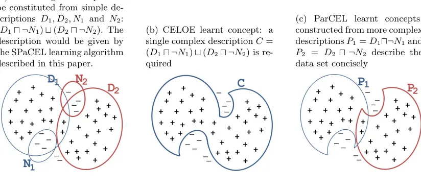
While this approach is suitable for many concept learning problems and has been used successfully by Hellmann (2008); Lehmann and Hitzler (2010); Tran et al. (2012), it does not use descriptions in the search space efficiently. Consider a top-down approach for learning such as CELOE, which constructs the search tree using a downward refinement operator until it finds a node (expression) that correctly and completely defines the positive examples. Given a concept learning problem with a set of positive (+) and negative (–) examples, the concepts D1, D2, N1, N2 and their coverage1 as described in Figure 1(a), CELOE will find the single concept C= (D1u ¬N1)t(D2u ¬N2) (shown in Figure 1(b)).
Algorithms that combine both top-down and bottom-up approaches (such as ParCEL and DL-FOIL) find two simpler concepts: P1 = D1 u ¬N1 and P2 = D2 u ¬N2. These concepts are visualised in Figure 1(c). If all of the concepts D1, D2, N1 and N2 have the same length of 3, then the length of the longest concepts generated by these two approaches are 16 (4 concepts of length 3 plus 4 operators) and 8 (2 concepts of length 3 plus 2 operators) respectively. If a concept is of length 16 then it must occur at a depth of at least 16 in the search tree, and so CELOE will only be able to identify this concept after searching the previous 15 levels of the search tree. As the expansion of the search tree in these approaches is directed by a heuristic that is based upon accuracy, not all branches of the search tree are fully expanded; this prevents ‘dummy’ breadth-first expansion.
The difference between these two methods is the way that the search tree is constructed: CELOE refines a general concept, while ParCEL searches for partial solutions that provide a correct (true) description of a subset of the data, and combines them to generate a complete solution. This idea of partial solutions can be extended to define exceptions as
Figure 1: Exception patterns in learning. Pluses (+) denote positive examples, minuses (–) denote negative examples. The ellipses represent coverage of the corresponding class expressions.
(a) The target concept can be constituted from simple de-scriptions D1, D2, N1 and N2: (D1u ¬N1)t(D2u ¬N2). The description would be given by the SPaCEL learning algorithm described in this paper.
(b) CELOE learnt concept: a single complex descriptionC= (D1u ¬N1)t(D2u ¬N2) is re-quired
(c) ParCEL learnt concepts: constructed from more complex descriptionsP1=D1u¬N1and P2 = D2 u ¬N2 describe the data set concisely
partial descriptions of negative examples, and this is what we consider in this paper. It enables a learning algorithm to find the solution suggested in Figure 1(a), which is at depth three in the search tree that combines descriptions of positive and negative examples separately. This is the main idea of the algorithm that we propose in this paper, which we call SPaCEL for reasons that will be made clear later, and which treats positive and negative examples equally and can search for their definition in parallel. Definitions of negative examples can then be combined with other concepts in the search tree to construct new partial solutions. In the case of the example in Figure 1, definitions N1 and N2 of negative examples, which are ignored by CELOE and ParCEL, are employed by SPaCEL and are combined with concepts D1 and D2 to to constitute partial solutions D1u ¬N1 (equivalent to P1 in CELOE) and D2u ¬N2 (equivalent toP2 in CELOE). In some cases, definitions of negative examples can be very simple and thus they can be found very early in the search process. In addition, each negative example can be combined with a variety of concepts to constitute several partial solutions. This will result in smaller search trees and faster learning time. Our evaluation shows that this approach works well not only in cases where exceptions exist, but also in normal cases.
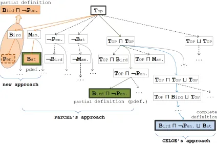
Figure 2, which extends theTweety example using the knowledge base shown in Figure 2(a), provides another simple example of the benefits of exceptions. For the instances given in Figure 2(b) (where bi are instances of Bird, pi instances of Penguin, ck instances of
Mammal and tm instances of Bat), the pi can be considered as exceptions to a rule that
says that birds fly, and likewise tm for a rule that says that mammals do not. Figure
Further, since some ‘useful’ definitions (such asBat in this example) are based on negative examples, they may be ignored by the first two approaches.
Another, more complex example that demonstrates differences between the three ap-proaches is in the uncle relationship for the Forte Uncle data set. The knowledge base of this data set contains concepts and relations that are related to family relationships, such as Person, Male, Female, married, has parent, has sibling, etc. It also includes some instances of people and their properties. For example,Alfred is a male and is the father of David and Elisa. Alice is a female, she is married to Art and is the mother of F14, M13, M15. Art is a male and he is the father of F14, M13 and M15. He also has two siblings, Umo and Wendy. Wendy is a female and is married to Walt. She has two children, F12 and M11. Her siblings are Art and Umo. In this set, Art is a positive example of an uncle, and Alfred, Alice and Wendy are negative examples (Alfred does not have siblings, Alice and Wendy are female). There are a total of 186 instances in the data set. A detailed description of this data set is provided in Section 3.1.
Written in Manchester syntax (Horridge and Patel-Schneider, 2009) and also in English, definitions of the uncle relationship learnt by the three different approaches are :
• CELOE:generates a single complex solution of length 15: male AND ((married SOME hasSibling SOME Person) OR
(married SOME hasSibling SOME hasChild SOME Thing))
(An uncle is a male who has married someone with a sibling; or a man who married someone’s sibling and the sibling has some children)
• ParCEL:generates two partial solutions of length 7 and 9: 1. male AND hasSibling SOME hasChild SOME Thing
(An uncle is a man who has at least sibling and a sibling has children)
2. male AND married SOME hasSibling SOME hasChild SOME Thing
(An uncle is a man who married someone with at least one sibling, and that sibling has a child)
• SPaCEL:generates two partial solutions that are created by combining two concepts “hasSibling SOME hasChild SOME Thing” of length 5 and “married SOME hasSi-bling SOME hasChild SOME Thing” of length 7 with a partial solution “female” of negative examples:
1. hasSibling SOME hasChild SOME Thing AND (NOT female)
(An uncle is a person who has a sibling with children, and who is not female)
Figure 2: Different approaches to learning the definition for the extended Tweety concept learning problem.
(a) The knowledge base of the learning
problem. (b) Visualisation of the knowledge base.
bi
(bird)
ck
(mammal)
pi(Pen.)
tm (Bat)
The partial solution of negative examples can be found in an early stage of the learning progress. However, it is ignored by CELOE and ParCEL, whereas SPaCEL employs it for later combinations with concepts in the search tree to generate partial solutions if possible. All three solutions are valid, but the SPaCEL one can be found more quickly.
Using exceptions could increase the risk of selective over-fitting, since sub-cases are given high weight, but the emphasis on short descriptions for the general rules, and the fact that the exception cases are also based on short descriptions, ensures that this is unlikely to happen. We present experimental evidence that this method often gives higher predictive accuracy on test data. It is true that logical formulae based on exceptions can quickly become torturous, as a short general description gets progressively more complex caveats added to it, and possibly even exceptions to the exceptions. However, the constraints on search that are implicit in logic programming (such as search tree size, definition length, and learning time) means that these complex cases are very unlikely to ever be found.
One key part of our approach is that positive and negative examples are treated in the same way; this ‘symmetry’ gives us the name of our algorithm: Symmetric Parallel Class Expression Learning (SPaCEL). A secondary point (referred to in the ‘parallel’ part of the name) is that the algorithm is inherently parallelisable in the first phase of learning, where separate definitions of positive and negative examples are sought. These definitions are combined in the second phase to construct a sufficiently accurate definition. By using rules about negative examples to remove them from the concepts in the search tree it is possible to combine (potentially very short) concepts and so define relatively complex concepts based on much smaller depth traversals. Consequently, concepts in the search tree are used more effectively and thus the learning time can be reduced.
We present a formal definition of our learning algorithm in Section 2, together with a discussion of various strategies for combining partial definitions of positive and negative examples. In addition, we demonstrate the parallelisation strategy that is one part of what makes our algorithm so effective computationally. We then present the data sets that we use for evaluation in Section 3.1, followed by a comparison of the three strategies for combining definitions that we have considered. Following this, in Section 3.3 we report search tree size, predictive accuracy, learning time, and definition length for 15 data sets of varying complexity for CELOE, ParCEL and SPaCEL. In Section 4.1, we summarise some related work before concluding with a summary and discussion of future work in Section 5. 2. Symmetric Parallel Class Expression Learning
Our learning approach constructs definitions of both positive and negative examples and gives them equal weight in order to find the final definition. This is performed in three main steps:
1. Find partial definitions for positive and negative examples separately such that the set of definitions, together, cover all positive and negative examples.
2. Consolidate the partial definitions to remove redundancies (i.e., the partial definitions whose coverage is a subset of the union of other partial definitions) and select the best candidates for constructing a complete definition.
In the first step, partial definitions can be produced directly by specialisation using a downward refinement operator, as in algorithms such as DL-FOIL and ParCEL. Definitions for negative examples are constructed side-by-side with definitions for positive examples and are used in combination with existing expressions in the search tree to create further partial definitions.
In the next section we introduce the concepts necessary for our algorithms. The al-gorithms themselves will be presented in Section 2.2. We follow the definitions used by Lehmann and Hitzler (2010) closely, although some of the concepts have to be extended in order to include negative examples.
2.1 Symmetric class expression learning
Aconcept learning problemin description logics can be described as a structurehK,(E+,E−)i where K is a knowledge base (ontology), E+ is a set of positive examples and E− is a set of negative examples such that E+∩ E− = ∅. A learnt concept is also called a hypothesis or definition. K |= C(a) denotes that a is an instance of class C with respect to the knowledge base K. If K |= C(a) is satisfied, C is said to cover a with respect to K. The aim of description logic learning is to find a concept C such that K |= C(e) for all e ∈ E+ (completeness) and K
2 C(e) for all e ∈ E− (correctness). A learnt concept is
called complete if it covers all positive examples, correct if it does not cover any negative examples, accurate if it is both complete and correct, overly general if it is complete but incorrect, and overly specific if it is correct but incomplete.
In order to define negative examples, we extend the concept cover for a set of instances in the form of a function, as follows:
Definition 1 (Cover) Let K be a logic knowledge base, X be a set of instances and C be a concept. Then, cover(K,C,X) is a function that computes a set of examples inX covered by Cwith respect to K:
cover(K,C,X) ={e∈ X | K |=C(e)(that is:eis covered by C with respect to K)}
This can be generalised to a set of definitions as: cover(K,Q,X) =S
C∈Qcover(K,C,X)
whereK be a knowledge base,X be a set of instances andQ be a set of definitions. Definition 1 enables us to give definitions of positive examples (which are called partial definitions) and negative examples (which are called counter-partial definitions):
Definition 2 (Partial definition) For a concept learning problem hK,(E+,E−)i, a con-cept C is called a partial definition if cover(K,C,E+)6=∅ and cover(K,C,E−) =∅.
Definition 3 (Counter-partial definition) For a concept learning problemhK,(E+,E−)i, a concept Cis called acounter-partial definitionifcover(K,C,E+) =∅andcover(K,C,E−)6=
Definitions 2 and 3 are ‘ideal’ in that they insist on the cover of the opposite set being the empty set. In practice, it is possible to allow a few negative examples to be covered by a partial definition, and a few positive examples by a counter-partial definition; this could potentially help with noisy data.
The first (top-down) step of our algorithm consists of finding partial and counter-partial definitions separately using a refinement operator and a combination strategy to compute further partial definitions from the counter-partial definitions and existing expressions in the search tree. As these searches are performed separately and simultaneously, our approach avoids being over-specific for concept learning problems that contain exceptions.
These sets are then combined, which enables the algorithm to cope with exceptions to general rules through the opposing definitions (so rules made of partial definitions can have counter-partial definitions added, and vice versa). This is simply the use of conjunction and negation, The combination acts as an extra step to deal with the exceptions with the support of counter-partial definitions. In our approach, only one downward refinement operator is used in the specialisation step to generate both partial and counter-partial definitions. The combination strategy essentially consists of checking for the possibility of creating new partial definitions from an expression and counter-partial definitions, using conjunction and negation: a combination of an expression C with a set of counter-partial definitionsX has the formCu ¬(tD∈XD).
Definition 4 (Combinability) Given a concept learning problem LP = hK,(E+,E−)i, a set of counter-partial definitionsQ, and an expression Csuch thatcover(K,C,E+)6=∅and cover(K,C,E−)=6 ∅, C is said to be combinable with Q iff:
cover(K,C,E−)⊆cover(K,Q,E−), which means that C can be “corrected” by Q.
The main objective of the combination step is to check for the combinability of descrip-tions in the search tree. Combining definidescrip-tions can be performed at several stages of the learning algorithm; this is discussed further in Section 2.3.
In this paper, we employ the refinement operator used by Lehmann and Hitzler (2010). However, the combination step helps us avoid the usage of negation in the refinement without any loss of generality, and the use ofpartial models and disjunction in the reduction steps means there is no need for disjunction in the refinement. Therefore, we use only 5 of the 7 basic rules in the original refinement operator described by Lehmann and Hitzler (2010). The two rules which refine the negation and disjunction are not used, thus our refinement operator is defined as:
Definition 5 (SPaCEL refinement operator ρu) Given an expression C, a set of con-cept names NC and a set of property (role) names NR, then ρu is defined as follows:
1. if C∈NC (C is an atomic concept):
ρu(C) ={C0 |C0 @C and @C00∈NC :C0 @C00@C} ∪ {CuC0 |C0 ∈ρu(>)}
2. if C=> (C is the TOP concept):
ρu(C) ={C0 |C0 ∈NC,@C00∈NC :C0@C00 @C} ∪ {∃r.> | r∈NR} ∪ {∀r.> | r∈NR}
(if C is the TOP concept, specialise it by using its proper sub-concepts or property restrictions)
3. if C=C1u...uCn (C is a conjunctive of descriptions):
ρu(C) ={C1u...uC0u...uCn |C0 ∈ρu(Ci),1≤i≤n}
(if C is a conjunction, it is specialised by refinements of its conjuncts)
4. if C=∀r.D, r∈NR: ρu(C) ={∀r.D0 | D0∈ρu(D)}
∪ {∀r.⊥ | D=A∈NC and @A0 ∈NC s.t. A0 @A}
(if C is a ‘for all’ property restriction, it is specialised by refinements of its range)
5. if C=∃r.D, r∈NR: ρu(C) ={∃r.D0 | D0∈ρu(D)}
(this rule is for the ‘there exists’ property restriction, and is similar to the4th rule.) Note that in the expression for ρu in the second rule, negation and disjunction are not used, since they can be generated by combination and aggregation (steps 2 and 3 of our algorithm) respectively.
The top-down step finishes when either the partial definitions cover all positive examples or the counter-partial definitions cover all negative examples (up to allowable noise), which produces this formal definition (where the first line of this describes as the union of correct descriptions of the positive data and correctable descriptions of the same data):
Definition 6 (SPaCEL top-down learning) Given a concept learning problem LP =
hK,(E+,E−)i, the top-down learning step in this approach aims to find a set of partial definitions P, a set of counter-partial definitions Q and a set of expressions X such that:
cover(K,P,E+)∪cover(K,X,E+) =E+,
such that∀C∈ X | C is combinable with Q, or cover(K,Q,E−) =E−.
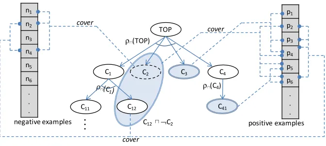
Figure 3 demonstrates the top-down step in our approach that uses the refinement operator ρu to produce both partial and counter-partial definitions. In this example, the combination of the counter-partial definition C2 and the expression C12 creates a partial definition C12u ¬C2.
As in the ParCEL algorithm, the selection of expressions in the search tree for refinement is controlled by node scores that are computed by a learning heuristic. The particular learning heuristic that we use is adapted from Lehmann and Hitzler (2010). However, the factors involving in the scoring function and their weights are redefined accordingly to our learning strategy:
Definition 7 (SPaCEL score) Let LP =hK,(E+,E−)i be a concept learning problem, C be a class expression and C0 the parent expression of C. The score of C is computed as:
score(C) = correctness(C, LP)
Figure 3: The top-down learning step aims to find both partial definitions and counter-partial definitions. Double-line nodes arepartial definitions,dashed-line nodes are counter-partial definitions. ρu is the refinement operator defined in Definition 5. Connections from nodes to examples represent thecoverage of the expressions.
ρ⊓(TOP)
TOP
C1 C4
C11 C12
ρ⊓(C4)
p1
p2
p3
p4
p5
p6
. . .
. .
.
C41
C2
positive examples n1
n2
n3
n4
n5
n6
. . .
negative examples
C3
C12⊓¬C2
cover
cover
cover
where gain(C, LP) =accuracy(C, LP)−accuracy(C0, LP).
In this definition, correctness, completeness and accuracy have their standard meanings, i.e., (Lehmann and Hitzler, 2010):
correctness(C, LP) = |E
−\cover(|K, C,E−)|
|E−| ,
completeness(C, LP) = |cover(K, C,E +)|
|E+| , accuracy(C, LP) = |cover(K, C,E
+)|+|E−\cover(K, C,E−)|
|E+∪ E−| .
The length of an expression is taken to be the sum of the number of concept names, role names, quantifiers, and connective symbols occurring in the expression, which for ex-pressions in the ALC language can be defined as:
Definition 8 (Length of an ALC expression) The length of an expressionDorE (de-noted by |D|) is defined inductively as follow (where A denotes an atomic concept):
|A|=|>|=|⊥|= 1
|¬D|=|D|+ 1
|D∪E|=|D∩E|= 1 +|D|+|E| |∃r.D|=|∀r.D|= 2 +|D|
expression is also applied, as accurate expressions are more likely to be close to the solution. A bonus is also given for the relatively complete expressions.
Default values for the weightings of the above factors were chosen based on experimental investigations and the work by Lehmann and Hitzler (2010). We chose α = 0.2, β = 0.01, γ = 0.05. These values can be adjusted based on the characteristics of the learning problem, such as decreasing the penalty for learning problems that need long definitions, thus biasing the search to look for deeper solutions.
The last step of our algorithm, the aggregation of the best candidates, can be performed using disjunction.
One optimisation step that can be applied to our learning is to noticeirrelevant concepts and remove them from the search tree. Irrelevant concepts are those from which no partial or counter-partial definition can be produced, hence they cannot be expanded. An irrelevant concept in SPaCEL is defined as follows:
Definition 9 (Irrelevant concept) Given a concept learning problem LP = hK,(E+,
E−)i, a concept C is irrelevant if cover(K, C,E+) = ∅ and cover(K, C,E−) = ∅, i.e., it covers no positive and no negative examples.
2.2 The algorithms
The SPaCEL learning algorithm is essentially top-down learning combined with a reduction task. The top-down step is used to solve the sub-problems of the given concept learning problem and the reduction is used to reduce and combine the sub-solutions into an overall solution. The former is performed by the downward refinement operator and a combination strategy, while the latter uses a set coverage algorithm to choose the best partial definitions and disjunction to form the overall solution.
Algorithm 1 describes the main loop of our learning algorithm, the reducer. It chooses the best concepts (i.e., those with highest score, based on the search heuristic described in Definition 7) from the search tree and uses theSpecialisealgorithm (see Algorithm 2) for refinement and evaluation until the completeness of the partial definitions is sufficient. Concepts are scored using an expansion heuristic that is mainly based on the correctness of the concepts. Our reducer is the analogue of the cover removal step in ILP in that it tries to remove redundancies.
The specialisation, which performs the refinement and evaluation of the concepts as-signed by the learning algorithm, is described in Algorithm 2. It refines the given concept (ρu(C)) and evaluates the result (cover(K, C,E+) andcover(K, C,E−)). Irrelevant concepts are removed, as no partial definition or counter-partial definition can be computed from them. Then, the specialisation finds new partial definitions, counter-partial definitions and descriptions from the refinements. In practice, new descriptions are checked for redun-dancy before being evaluated and added to the search tree, as the same description can be generated from different branches of the search tree.
Algorithm 1:Symmetric Class Expression Learning Algorithm– SPaCEL(K,E+,E−, ε)
Input: background knowledgeK, a set of positiveE+ and negative E− examples, and a noise valueε∈[0,1] (0 means no noise)
Output: a definitionC such that|cover(K, C,E+)| ≥(|E+| ×(1−ε)) andcover(K, C,E−) =∅ (empty set)
1 begin
2 initialise the search treeST ={>} /* >: TOP concept in DL */
3 cum pdefs =∅ /* set of cumulative partial definitions */
4 cum cpdefs =∅ /* set of cumulative counter-partial definitions */
5 cum cp=∅ /* set of cumulative covered positive examples */
6 cum cn=∅ /* set of cumulative covered negative examples */
/* cf. Def. 6 for the meaning of the OR operator */
7 while|cum cp|<(|E+| ×(1−ε))or |cum cn|<|E−|do
8 get and remove the ‘best’ conceptB fromST /* see text */
9 (pdefs,cpdefs, descriptions) =Specialise(B,E+,E−) /* cf.Alg.2 */
10 cum pdefs=cum pdefs ∪pdefs 11 cum cpdefs=cum cpdefs ∪cpdefs
12 cum cp=cum cp∪ {e|e∈cover(K, P,E+), P ∈pdefs} 13 cum cn=cum cn∪ {e|e∈cover(K, P,E−),P∈cpdefs}
/* online combination, see Sec.2.3 */
14 foreachD ∈ descriptions do
/* if D can be ‘‘corrected’’ by existing cpdefs */
15 if (cover(K, D,E−) \ cum cn) =∅ then
/* combine D with cpdefs if possible */
16 candidates=Combine(D,cum cpdefs,E−) /* cf.Alg.3 */
17 new pdef=Du ¬(FA∈candidates(A)) /* new partial def. */
18 cum pdefs=cum pdefs ∪new pdef
19 cum cp=cum cp∪cover(K,new pdef,E+)
20 else
21 ST =ST∪ {D}
/* explore more partial definitions to satisfy completeness */
22 if |cum cp|<(|E+| ×(1−ε))then
23 foreachD∈ST do
24 candidates=Combine(D,cum cpdefs,E−) 25 new pdef=Du ¬(FA∈candidates(A))
26 cum pdefs=cum pdefs ∪new pdef
where possible, a form of theory learning. Concepts that have been refined can be scheduled for further refinements.
The refinement operator given in Definition 5 is infinite (i.e., it can continue to expand the tree without limit), but in practice each refinement step is monotonic and bounded, as it is only allowed to generate descriptions of at most a pre-defined length (see Definition 8). For example, a concept of lengthN will first be refined to concepts of length (N + 1), and later, when it is revisited, to concepts of length (N+2), etc. For the sake of simplicity, we use ρu in the algorithms to refer to one refinement step rather than the entire refinement. This technique is used in DL-Learner and discussed in detail by Lehmann and Hitzler (2010).
When the learning algorithm reaches a sufficient degree of completeness, it stops and reduces the partial definitions to remove the redundancies using the Reduce function, which is essentially a set coverage algorithm: given a set of partial definitionsX and a set of positive examplesE+, it finds a subsetX0 ⊆ X such thatE+⊆S
D∈X0(cover(K, D,E+)).
The solution returned by the algorithm is a disjunction of the reduced partial definitions. As an alternative, a set of partial definitions could be returned instead. This may be useful in some contexts, such as making the result more readable. The reduction algorithm may be tailored to meet particular requirements, such as the shortest definition or the smallest number of partial definitions. The combination of descriptions and counter-partial definitions that is given in Algorithm 1 is one of the combination strategies implemented in our evaluation. This strategy is called theon-the-fly combination strategy; it gave the best performance in our evaluation (see Section 3.2). A description of the various combination strategies we tried is given in Section 2.3.
Algorithm 2:Specialisation algorithm –Specialise(C,K,E+,E−)
Input: a descriptionC and a concept learning problem LP =hK,(E+,E−)i. Output: a triple consisting of a set of partial definitionspdefs ⊆ρu(C); a set of
counter-partial definitions cpdefs ⊆ρu(C); and a set of new descriptions descriptions ⊆ρu(C) such that
∀D∈descriptions:Dis not irrelevant and D /∈(pdefs∪cpdefs), in which ρu is the refinement operator defined in Definition 5.
1 begin
2 pdefs = {D∈ρu(C) |cover(K, D,E+)6=∅ ∧ cover(K, D,E−) =∅} 3 cpdefs ={D∈ρu(C) |cover(K, D,E+) =∅ ∧ cover(K, D,E−)6=∅} 4 descriptions = {D∈ρu(C) |cover(K, D,E+)6=∅ ∧ cover(K, D,E−)6=∅} 5 return(pdefs, cpdefs, descriptions)
Algorithm 3:Combination algorithm –Combine(C,cpdefs,E−)
Input: a description C, a set of counter-partial definitionscpdefs and a set of negative examplesE−
Output: a setcandidates ⊆cpdefs such that cover(K, C,E−)⊆S
P∈candidates(cover(K, P,E−)) 1 begin
2 candidates = ∅ /* candidate counter-partial definitions */
3 cn c=cover(K, C,E−) /* negative examples covered by C */
4 sortcpdefs by descending coverage of negative examples 5 whilecpdefs6=∅ andcn c6=∅ do
6 get and remove the top counter-partial definitionD fromcpdefs 7 if (cover(K, D,E−)∩cn c)6=∅ then
8 candidates=candidates∪D 9 cn c=cn c\cover(K, D,E−)) 10 if cn c6=∅then
11 return∅ /* return the empty set */
12 else
13 returncandidates
Completeness of the algorithm
The refinement operator used in our algorithm is based on the refinement operator described by Lehmann (2010). In that paper a proof of completeness over theALC language is given, i.e., any concepts in the ALC language can be produced by this operator after a finite number of refinement steps.
Due to our learning strategy, our refinement operator does not generate negation and disjunction. As a result, our refinement operator itself is not complete. However, negation and disjunction can be created by the reduction and combination steps of the algorithm. The combination step uses negation and conjunction to correct an expression with counter-partial definitions (see Algorithm 3 and Definition 4) whereas the reduction step can gener-ate disjunctions. Clearly, the completeness of our algorithm depends upon the combination strategy that produces the negations. Three combination strategies are proposed in Section 2.3, and our learning algorithm is complete when the on-the-fly and delayed combination strategies are used; completeness is not guaranteed for thelatecombination strategy. 2.3 Counter-partial definitions combination strategies
2.3.1 Late combination
In this strategy, the algorithm maintains sets of partial definitions and counter-partial defini-tions separately. When all positive or negative examples are covered (or another termination condition is reached, such as maximum time allowed, or a sufficient percentage of examples covered), it will combine descriptions from the search tree and the set of counter-partial definitions.
Since the combination is performed after the learning stops, this strategy may provide a better combination, i.e., it may have better choices of counter-partial definitions to use for the combination. However, for concept learning problems in which both positive and negative examples use negation, the algorithm may not be able to find the definition because the refinement operator designed for this algorithm does not use negation. If this is the case and a maximum time timeout is set, then the combination will be made when the timeout is reached in order to find the definition. Otherwise, the algorithm will not terminate.
For example, the concept learning problem shown in Figure 2 may cause this strategy to run out of memory without finding an accurate concept if there is no timeout or no noise is allowed. To cover all positive examples, we need a class expression with negation as follows:
Batt (Birdu ¬Penguin)
and to completely cover all negative examples, the following class expression is needed: Penguint (Mammalu ¬Bat)
To produce the definition for positive examples, the counter-partial definitionPenguin
needs to be combined with the expression Bird, which cannot be performed directly due to the removal of negation from the refinement operator. However, in this strategy, the combination is only called when all positive examples or negative examples are covered, and in the example this condition is never met, as the expression ¬Batcannot be produced. 2.3.2 On-the-fly combination
This strategy is used in Algorithm 1. When a new description is generated from the refine-ment or an existing description is revisited, it is combined with the existing counter-partial definitions if possible. This strategy can avoid the termination problem discussed in thelate combination strategy because negation is used in the combination. The evaluation suggests that this strategy, overall, gives the best performance and the smallest search tree. However, the final results can be optimised since a counter-partial definition may be combined with many expressions and thus the final definition is unnecessarily long. For example, in the concept learning problem described in Figure 2, when the description Bird is generated, there is no counter-partial definition to combine it with. However, when it is revisited for refinement, it will be combined with the new counter-partial definitionPenguinto produce a partial definitionBirdu ¬Penguin.
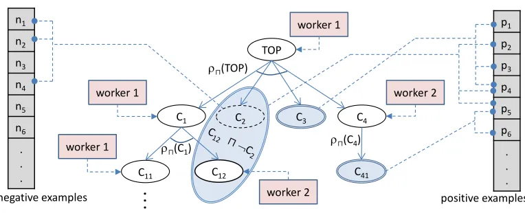
counter-Figure 4: Top-down learning in SPaCEL with multiple workers.
ρ⊓(TOP)
ρ⊓(C1)
TOP
C1 C4
C11 C12
ρ⊓(C4) worker 1
worker 1
worker 1
worker 2
p1 p2 p3 p4 p5 p6 . . . worker 2
C3
. .
.
C41 C2
positive examples n1
n2 n3 n4 n5 n6 . . .
negative examples
partial-definitions are stored to be reused to “correct” the new descriptions in the search tree, while the original refinement may regenerate the same negated description.
2.3.3 Delayed combination
This strategy lies inbetween the previous two, and checks the possibility of combinations when a new description is generated. However, even if the combination is possible, only the set of cumulative covered positive examples is updated (by removing the elements that are covered by the new description), while the new description is put into a potential partial definitions set. The combination is executed when the termination condition is reached, i.e., either all positive examples or all negative examples are covered, or the algorithms times out.
This strategy may help to prevent the problem of the late combination strategy, and it may return better combinations in comparison with the on-the-fly strategy because it inherits the advantage of the late combination strategy. However, as the combinable de-scriptions in this strategy are not combined until the learning terminates, the search tree is likely to be larger than that of the on-the-fly strategy.
2.4 Parallelisation of the learning algorithm
One benefit of the symmetric approach is that it is inherently parallel: several expressions (branches) in the search tree can be processed (refined and evaluated) in parallel using multiple workers to find the partial definitions. A central reducer, which is part of the learner, controls the management of partial and counter-partial definitions produced by the workers until the termination condition described in Definition 6 is met. Then it performs the reduction and aggregation steps to create a final definition. The parallel exploration of the search tree by multiple workers is illustrated in Figure 4.
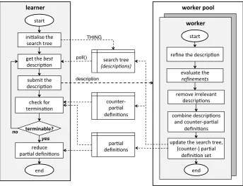
Figure 5: Implementation architecture. Note that the combination step may be performed by the workers or the reducer, depending upon the combination strategy (see Section 2.3).
worker pool
worker
start
refine the descrip.on
evaluate the refinements
end search tree
(descrip.ons)
learner
start
check for termina.on
terminable?
end no
ini.alise the search tree
get the best descrip.on
submit the descrip.on
counter-‐ par.al defini.ons
reduce par.al defini.ons
par.al defini.ons
THING
poll()
remove irrelevant descrip.ons
combine descrip.ons and counter-‐par.al
defini.ons
update the search tree, (counter-‐) par.al
defini.on set yes
description
done by the multiple workers. The combining of descriptions and counter-partial definitions is also performed on the worker side.
3. Evaluation
In order to evaluate the Symmetric Class Expression Learning approach of SPaCEL, we compared it to CELOE and ParCEL using 10-fold cross validation with 15 data sets. These are summarised in Section 3.1, using the search tree size, predictive accuracy and learning time, and the length of the definitions learnt as the metrics for comparison. CELOE is one of the description logic learning algorithms in the DL-Learner framework. It is well-evaluated and has been compared with many other learning algorithms. Therefore, using it for com-parison enables an implicit comcom-parison with other learning algorithms; the evaluations by Hellmann (2008); Lehmann (2010) suggest that, overall, CELOE produced better results than the comparators. The implementation of CELOE that we used is publicly available athttps://github.com/tcanvn/SParCEL/.
3.1 Experimental data sets
To ensure the evaluation covers as much as possible of the space of cases, which helps to archive a thorough assessment of the learning algorithms, we chose data sets that vary in: i) size of knowledge base and examples, ii) the length of definitions, and iii) the amount of noise. In some cases, (i) was achieved by using subsets of a particular data set.
The data sets are divided into three groups. The first group includes 7 learning problems that have low to medium complexity and on which all algorithms in the experiment can find solutions on the training set without timing out in the 10 minutes we allowed. The second group contains high to very high complexity learning problems; all algorithms in the experiment can also find accurate solutions on the training set without timing out. The third contains leaning problems for which one of the learning algorithms could not find accurate solution on the training set (i.e. timeout occurred). The complexity of the learning problems is approximately estimated based on the definition length produced by CELOE: i) low: (0, 8]; ii) medium: (8, 15]; iii) high: (15, 20]; and very high: longer than 20. The reason for treating problems learnt with and without timeout separately is that some metrics cannot be compared if the learning algorithm cannot find the solution (e.g. learning time, search space size).
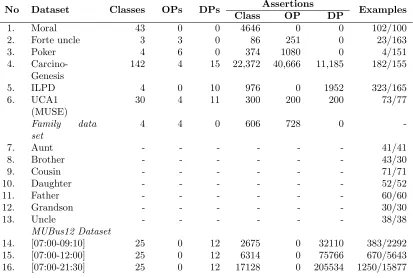
The list of data sets used and their properties are summarised in Table 1, and an overview of them is given next. We use Manchester OWL Syntax (Horridge and Patel-Schneider, 2009) to describe the learning problems’ expected definitions.
Moral This data set was first introduced by Wogulis (1994) and is available at the Uni-versity of California Irvine (UCI) machine learning repository2 (Frank and Asuncion, 2010). It is intended to be used to learn definitions of harm-doing activities and con-tains concepts and observations related to the classification of activities as ‘guilty’ and ‘not guilty’ through a set of sub-categories such as ‘blameworthy’ and ‘justified’. Poker A description of 10 classes of poker hands (5 cards drawn from a standard deck)
based on 10 predictive attributes (suit and rank of each card). This data set can be customised into binary-class learning and is available at the UCI repository3.
Family A set of data sets containing observations about family relations such as aunt, brother, cousin, daughter, father, grandson and uncle (Richards and Mooney, 1995). This data set can be found in many repositories. In our evaluation, we use the data set distributed with the DL-Learner package (which can be found in the DL-Learner repository4). Each family relation can be treated as a separate learning problem, and we use several of them. We also use the Forte Uncle problem used by Lehmann (2007) and available in the DL-Leaner repository.
CarcinoGenesis This data set is used to learn the structure of chemical compounds and bioassays that may cause cancer based on data from the US National Toxicology Program. It was transformed into logic programming and used for evaluation of ILP algorithms by many authors such as Bahler (1993); Srinivasan et al. (1997) and was 2. http://archive.ics.uci.edu/ml/datasets/Moral+Reasoner
transformed into the OWL ontology format and used to evaluate the description logic learning algorithms in the DL-Learner framework (Lehmann, 2010)5. It is particularly noisy, which makes it a challenging problem in machine learning for both symbolic and sub-symbolic learning approaches.
MUSE Dataset We employ use case 1 of a set of context-aware smart home simulations by Lyons et al. (2010) for normal and abnormal living behaviours. The data set is available in the SPaCEL repository6.
ILPD Dataset A data set based on the liver function test records of patients collected from the North East of Andhra Pradesh, India (Indian Liver Patient Dataset). Each record comprises patient information such as age and gender and results of liver function tests including total Bilirubin, Albumin, and total protein, and the target is an expert-assigned label of cancerous or non-cancerous. This data set is also available in the UCI repository7.
MUBus Dataset A data set developed to demonstrate the SPaCEL algorithm, it is based on a bus timetable that varies according to conditions such as weekday/weekend, uni-versity holidays, and school holidays. Data was generated by sampling at 5 minute intervals. Sub-datasets can be created by restricting the sampling times, such as “MUBus12 [07:00 - 09:20]” (shortened as MUBus-1), “MUBus12 [07:00 - 12:00]” (shortened as MUBus-2) and “MUBus12 [07:00 - 21:30]” (shortened as MUBus-3). This data set is available in the SPaCEL repository; for more information about it, see (Tran, 2013).
The timetable makes surprising complicated rules, such as the following description for a weekend bus:
(NOT Holiday1) AND ((hasMinute VALUE 0 and hasHour VALUE 9) OR (hasMinute VALUE 20 AND
(hasHour VALUE 10 OR hasHour VALUE 14 OR hasHour VALUE 16)) OR (hasMinute VALUE 40 AND
(hasHour VALUE 11 OR hasHour VALUE 13 OR hasHour VALUE 15)))
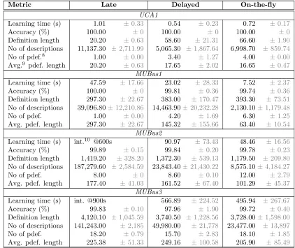
3.2 Comparison of Combination Strategies
As was described in Section 2.3, three combination strategies were implemented: late, de-layed and on-the-fly. We chose to compare these strategies in order to choose one as the most useful for SPaCEL. Table 2 shows the experimental results. It can be seen that the accuracies achieved are similar across all three, but the learning times and search space sizes differ. For example, the late combination strategy did not terminate in some cases: for the MUBus-2 data set the learner was interrupted by timeout after 10 minutes. However, by applying the algorithm after the learner was interrupted, a definition with 100% accuracy on the training data set was produced. This means the solution existed implicitly, but the
5. http://svn.code.sf.net/p/dl-learner/code/trunk/examples/carcinogenesis/ 6. https://github.com/tcanvn/SParCEL/
Table 1: Properties of the evaluation data sets. OPs and DPs are short for Object Properties and Data Properties respectively. Number of examples is given in the form positive/negative examples.
No Dataset Classes OPs DPs Assertions Examples
Class OP DP
1. Moral 43 0 0 4646 0 0 102/100
2. Forte uncle 3 3 0 86 251 0 23/163
3. Poker 4 6 0 374 1080 0 4/151
4. Carcino-Genesis
142 4 15 22,372 40,666 11,185 182/155
5. ILPD 4 0 10 976 0 1952 323/165
6. UCA1 (MUSE)
30 4 11 300 200 200 73/77
Family data set
4 4 0 606 728 0
-7. Aunt - - - 41/41
8. Brother - - - 43/30
9. Cousin - - - 71/71
10. Daughter - - - 52/52
11. Father - - - 60/60
12. Grandson - - - 30/30
13. Uncle - - - 38/38
MUBus12 Dataset
learner was not able to compute it. To make sure that the learner was not terminated too early, the experiment was rerun for 3 hours, but the learner was still not able to find the solution on the training data set. This demonstrates the disadvantage of this strategy. Table 2: Combination strategies experimental result (means ± standard deviations of 10 folds).
Metric Late Delayed On-the-fly
UCA1
Learning time (s) 1.01 ±0.33 0.54 ±0.23 0.72 ±0.17 Accuracy (%) 100.00 ±0 100.00 ±0 100.00 ±0 Definition length 20.20 ±0.63 58.60 ±21.31 66.60 ±1.90 No of descriptions 11,137.30 ±2,711.99 5,065.30 ±1,867.64 6,998.70 ±859.74 No of pdef.8 1.00 ±0.00 3.40 ±1.27 4.00 ±0.00 Avg.9 pdef. length 20.20 ±0.63 17.65 ±2.02 16.65 ±0.47
MUBus1
Learning time (s) 47.59 ±17.66 23.02 ±28.33 7.52 ±2.37 Accuracy (%) 100.00 ±0 99.81 ±0.36 99.74 ±0.36 Definition length 297.30 ±22.67 383.00 ±170.47 393.30 ±73.51 No of descriptions 39,096.80±12,210.86 14,463.90±20,232.28 2,130.10±1,179.48 No of pdef. 1.00 ±0.00 4.20 ±1.69 6.30 ±1.25 Avg. pdef. length 297.30 ±22.67 145.32 ±155.66 63.40 ±10.54
MUBus2
Learning time (s) int.10 @600s 90.97 ±73.43 48.46 ±16.56
Accuracy (%) 99.89 ±0.15 99.84 ±0.20 99.78 ±0.23 Definition length 1,419.20 ±328.20 1,372.30 ±539.13 1,179.50 ±209.80 No of descriptions 187,279.60 ±2,584.59 23,843.40±21,430.22 8,575.10±4,184.27 No of pdef. 8.00 ±0 8.60 ±0.10 12.00 ±2.79 Avg. pdef. length 177.40 ±41.03 161.52 ±67.40 101.29 ±45.37
MUBus3
Learning time (s) int. @900s 566.89 ±224.52 495.94 ±267.67 Accuracy (%) 99.83 ±0.10 97.96 ±1.90 99.72 ±0.40 Definition length 4,120.10 ±1,045.59 3,740.50 ±1,228.56 3,728.00±1,598.00 No of descriptions 141,243.00 ±2,185 49,980.00 ±21,778 23,477.00 ±13,897 No of pdef. 18.20 ±0.79 15.70 ±2.83 18.10 ±1.85 Avg. pdef. length 225.38 ±51.33 249.16 ±100.58 205.90 ±85.49
In addition, as the late combination strategy performed the combination at the end, only after all positive or negative examples are covered, its learning times were always longer than other strategies. In theory this might produce more concise solutions than the on-the-fly strategy, as can be seen in the following partial definitions produced by the on-the-on-the-fly strategy with the UCA1 data set:
1. activityHasDuration SOME hasDurationValue≤15.5 AND
(NOT (Activity AND activityHasDuration SOME hasDurationValue≤4.5))
8. Partial definitions 9. Average
2. activityHasStarttime SOME Autumn AND
(NOT (Activity AND activityHasDuration SOME hasDurationValue≤4.5)) AND (NOT (Activity AND activityHasDuration SOME hasDurationValue≥19.5))
3. activityHasStarttime SOME Summer AND
(NOT (Activity AND activityHasDuration SOME hasDurationValue≤4.5)) AND (NOT (Activity AND activityHasDuration SOME hasDurationValue≥19.5))
4. activityHasDuration SOME hasDurationValue≥4.5 AND activityHasStarttime SOME Spring AND
(NOT (Activity AND activityHasDuration SOME hasDurationValue≥19.5))
In contrast, the delayed strategy found:
activityHasDuration SOME (hasDurationValue≥4.5 AND hasDurationValue≤19.5) AND
(NOT (activityHasStarttime SOME Winter AND
activityHasDuration SOME hasDurationValue≥15.5))
The difference is between a large number of short expressions and a smaller number of long ones; usually the delayed strategy produced shorter descriptions overall. However, the on-the-fly strategy dominated in most aspects, particularly the learning time and search space covered. Our hope that the delayed strategy would combine the advantages of both of the others was not bourne out, and we therefore chose to use the on-the-fly strategy for the experimental comparison of SPaCEL with other algorithms.
3.3 Comparison Experiment
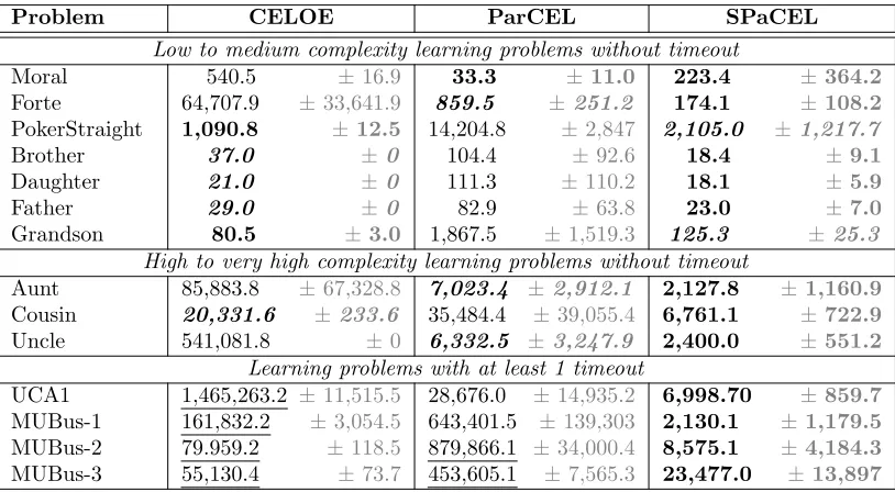
We measured search tree size (Table 3), predictive accuracy (Table 4), learning time (also Table 4), and definition length (Table 6) for all 15 data sets using CELOE, PaRCEL and SPaCEL. This section reports and discusses the results of this experiment.
The search tree size reported in this experiment is the total number of all descriptions that are inserted into the search tree, including the irrelevant descriptions (the partial and counter-partial definitions which are removed later by the algorithm). If an algorithm can find the solution, the result reported is the search tree size after the learning algorithm has terminated. Otherwise, it is the search tree size at the time when the timeout has occurred. In this case, the comparison should be treated with caution as it depends upon the timeout assigned for the learning algorithm. Only learning problems on which at least one of the algorithms found an accurate definition on the training set were considered. Therefore, the results for the CarcinoGenesis and ILDP learning problems are not reported, since all three algorithms timed out.
Table 3: Search tree size (means ±standard deviations of 10 folds). The underlined values are the search tree size after thetimeouthas occurred. The statistical significance was tested using t-tests: bold values are statistically significantly higher (at the 95% confidence level) than other values; unformatted values are statistically significantly lower than other values; bold italic values are statistically significantly lower than the bold values, and statistically significantly higher than the unformatted values.
Problem CELOE ParCEL SPaCEL
Low to medium complexity learning problems without timeout
Moral 540.5 ±16.9 33.3 ±11.0 223.4 ±364.2
Forte 64,707.9 ±33,641.9 859.5 ±251.2 174.1 ±108.2
PokerStraight 1,090.8 ±12.5 14,204.8 ±2,847 2,105.0 ±1,217.7
Brother 37.0 ±0 104.4 ±92.6 18.4 ±9.1
Daughter 21.0 ±0 111.3 ±110.2 18.1 ±5.9
Father 29.0 ±0 82.9 ±63.8 23.0 ±7.0
Grandson 80.5 ±3.0 1,867.5 ±1,519.3 125.3 ±25.3 High to very high complexity learning problems without timeout
Aunt 85,883.8 ±67,328.8 7,023.4 ±2,912.1 2,127.8 ±1,160.9
Cousin 20,331.6 ±233.6 35,484.4 ±39,055.4 6,761.1 ±722.9
Uncle 541,081.8 ±0 6,332.5 ±3,247.9 2,400.0 ±551.2 Learning problems with at least 1 timeout
UCA1 1,465,263.2 ±11,515.5 28,676.0 ±14,935.2 6,998.70 ±859.7
MUBus-1 161,832.2 ±3,054.5 643,401.5 ±139,303 2,130.1 ±1,179.5
MUBus-2 79.959.2 ±118.5 879,866.1 ±34,000.4 8,575.1 ±4,184.3
expanded redundantly and thus the reported search tree sizes might be unnecessarily larger than the minimal search tree size required to learn the problem.
In the second and the third groups, SPaCEL always produced the smallest search trees for all learning problems. The search tree sizes generated by the three algorithms for the same learning problem in this group were extremely different. For example, SPaCEL only needed to explore about 2,400 expressions to find the solution for the Uncle learning problem while CELOE had to explore more than 541,081 expressions. Similarly, SPaCEL found a solution after exploring about 2,130 expressions, while ParCEL needed to explore 643,401 expressions on the MUBus-1 learning problem. CELOE could not find an accurate solution for this learning problem and timed out after 10 minutes. The average search tree size at the time of timeout was about 161,832 expressions.
A t-test rejected the null hypothesis for similarity of search tree size of the algorithms on all learning problems at the 99% confidence level, meaning that the search trees generated by SPaCEL were statistically significantly smaller than CELOE in 12 out of 14 learning problems and than ParCEL for 13 out of 14 learning problems.
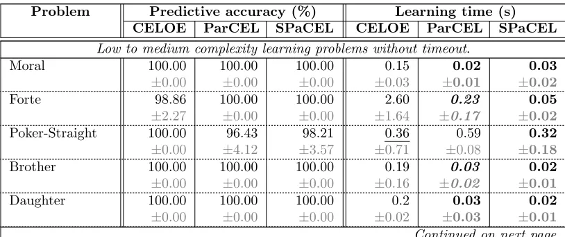
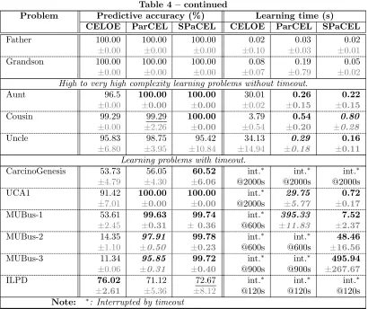
With regard to predictive accuracy and learning time, which are reported in Table 4, in general, SPaCEL achieved better predictive accuracy in most learning problems. In the first two groups (10 learning problems) all three learning algorithms achieved very high accuracy, including 100% accuracy in 5 of them. In the remaining 5 learning problems, SPaCEL was statistically significantly more accurate than CELOE for 3 out of 5 and ParCEL for 1 out of 5 problems. There were no learning problems in this group where SPaCEL was statistically significantly less accurate than either of the other algorithms.
Table 4: Learning time and predictive accuracy experimental results summary (means ±
standard deviations of 10 folds). Result of the statistical significance t-test (at the 95% confidence level) is also included: the bold and highlighted values are statistically signifi-cantlybetter than other values; the unformatted values are statistically significantly worse than other values; the bold and italic and highlighted values are statistically significantly worse than the bold and highlighted values, and statistically significantly better than the unformatted values; the underlined values represent the values that are not statistically significantly different from the other values.
Problem Predictive accuracy (%) Learning time (s)
CELOE ParCEL SPaCEL CELOE ParCEL SPaCEL
Low to medium complexity learning problems without timeout.
Table 4 – continued
Problem Predictive accuracy (%) Learning time (s)
CELOE ParCEL SPaCEL CELOE ParCEL SPaCEL
Father 100.00 ±0.00 100.00 ±0.00 100.00 ±0.00 0.02 ±0.10 0.03 ±0.03 0.02 ±0.01 Grandson 100.00 ±0.00 100.00 ±0.00 100.00 ±0.00 0.08 ±0.07 0.19 ±0.79 0.05 ±0.02 High to very high complexity learning problems without timeout.
Aunt 96.5 ±0.00 100.00 ±0.00 100.00 ±0.00 30.01 ±0.02 0.26 ±0.15 0.22 ±0.15 Cousin 99.29 ±0.00 99.29 ±2.26 100.00 ±0.00 3.79 ±0.54 0.54 ±0.20 0.80 ±0.28 Uncle 95.83 ±6.80 98.75 ±3.95 95.42 ±10.84 34.13 ±14.94 0.29 ±0.18 0.16 ±0.11 Learning problems with timeout.
CarcinoGenesis 53.73 ±4.79 56.05 ±4.30 60.52 ±6.06 int.∗ @2000s int.∗ @2000s int.∗ @2000s UCA1 91.42 ±7.01 100.00 ±0.00 100.00 ±0.00 int.∗ @2000s 29.75 ±5.77 0.72 ±0.17 MUBus-1 53.61 ±2.45 99.63 ±0.31 99.74 ±0.36 int.∗ @600s 395.33 ±11.83 7.52 ±2.37 MUBus-2 14.35 ±1.10 97.91 ±0.50 99.78 ±0.23 int.∗ @600s int.∗ @600s 48.46 ±16.56 MUBus-3 11.34 ±0.06 95.85 ±0.31 99.72 ±0.40 int.∗ @900s int.∗ @900s 495.94 ±267.67 ILPD 76.02 ±2.61 71.12 ±5.36 72.67 ±8.12 int.∗ @120s int.∗ @120s int.∗ @120s Note: ∗: Interrupted by timeout
In the last group of problems SPaCEL outperformed CELOE on 5 out of 6 and ParCEL on 3 out of 6 learning problems. The data set MU-Bus is a complex learning problem in which the target definition is very long, as the bus operation time depends upon many conditions. For this data set, SPaCEL outperformed both ParCEL and CELOE. It always found the complete definition on the training set and the accuracy on the test set was always over 99.7%, while CELOE could not find accurate definitions on the training set and the accuracy on the test set was very low, from 11.34% to 53.61%. ParCEL performed better than CELOE and the accuracy was also very high but it was still statistically significantly less accurate than SPaCEL.
For the ILPD data set it appears that CELOE had higher predictive accuracy that SPaCEL, although the difference was not statistically significant. However, as the ILPD and MuBus data sets are unbalanced, it is more appropriate to use balanced accuracy11for these learning problems. Table 5 shows the balanced predictive accuracy for ILPD and some other unbalanced learning problems. The balanced accuracy of SPaCEL and ParCEL on the ILDP learning problem were statistically significantly higher than CELOE. The outcome of the statistical significance test on the balanced accuracy of other learning problems did not change.
11.balanced accuracy = 1 2 ·
|true positive| |positive examples| +
|true negative| |negative examples|
Table 5: Balanced predictive accuracy of unbalanced data sets in Table 4. Conventions of the results’ representation are similar to that of in Table 4.
Problem Balanced predictive accuracy (%)
CELOE ParCEL SPaCEL
MUBus-1 71.12 ±0.65 99.68 ±0.60 99.74 ±0.62
MUBus-2 52.09 ±0.06 91.86 ±3.02 99.78 ±0.59
MUBus-3 52.18 ±0.03 73.07 ±1.91 99.02 ±2.67
ILDP 64.62 ±4.83 70.94 ±10.87 71.73 ±12.29
Our symmetric approach to class expression learning not only increased the predictive accuracy, but also decreased the learning time, although this effect can only be observed for the medium and high complexity data sets. The t-test result on learning time shows that SPaCEL was statistically significantly faster than CELOE in 13 out of 14 problems and than ParCEL for 10 out of 14 learning problems. It was statistically significantly slower than ParCEL for 2 out of 14 problems, both in the first and second groups. The definition lengths in this group were short and the learning times were very small.
The last metric that we evaluated was the length of the definitions learnt; the results can be seen in Table 6. The definition lengths of ParCEL and SPaCEL are reported by the number of partial definitions and the average length of the partial definitions, the total average length of their definitions is the product of those numbers.
Table 6: Definition length of the learning problems (means ± standard deviations of 10 folds). The bold values are the definition lengths after the timeout occurred.
Problem (Partial) definition length No of partial definitions
CELOE ParCEL SPaCEL ParCEL SPaCEL
Low to medium complexity learning problems without timeout
Moral 3.00 ±0.00 1.52 ±0.05 1.50 ±0.00 2.10 ±0.32 2.00 ±0.00 Forte 13.50 ±1.00 7.75 ±0.50 8.50 ±0.00 2.00 ±0.00 2.00 ±0.00 PokerStraight 11.70 ±0.68 10.90 ±1.31 19.75 ±2.50 1.70 ±0.68 1.00 ±0.00 Brother 6.00 ±0.00 6.00 ±1.83 6.40 ±0.84 1.00 ±0.00 1.00 ±0.00 Daughter 5.00 ±0.00 5.25 ±1.09 6.20 ±0.63 1.10 ±0.32 1.00 ±0.00 Father 5.00 ±0.00 5.50 ±0.53 5.90 ±0.98 1.00 ±0.00 1.00 ±1.00 Grandson 7.25 ±0.50 7.25 ±0.50 8.00 ±0.00 1.00 ±0.00 1.00 ±0.00 High to very high complexity learning problems without timeout
Table 6 – continued
Problem (Partial) definition length No of partial definitions
CELOE ParCEL SPaCEL ParCEL SPaCEL
Uncle 19.00 ±14.94 8.40 ±0.38 10.15 ±1.67 2.00 ±0.00 2.00 ±0.00 Learning problems with timeout
CarcinoGenesis 4.80 ±0.42 55.87 ±9.52 138.00 ±51.46 72.70 ±3.43 17.00 ±5.74 UCA1 9.00 ±0.00 12.75 ±0.00 16.65 ±0.47 4.00 ±0.00 4.00 ±0.00 MUBus-1 12.70 ±0.48 16.99 ±0.42 63.40 ±10.54 15.00 ±1.56 6.30 ±1.25 MUBus-2 2.00 ±0.00 16.07 ±0.19 101.29 ±45.37 24.80 ±3.52 12.00 ±2.79 MUBus-3 2.00 ±0.00 14.64 ±0.13 205.90 ±85.49 25.40 ±1.58 18.10 ±1.85 ILPD 5.80 ±1.69 8.34 ±0.12 13.30 ±1.40 42.80 ±1.69 37.00 ±2.06
The experimental results show that ParCEL and SPaCEL produced longer definitions than CELOE for most learning problems. By manually inspecting the results we identified that this was because partial definitions tend to overlap, and that the creation of sub-solutions leads to more specific definitions. It may also be that since CELOE timed out more often, it had not yet managed to produce completely accurate (and necessarily longer) solutions before the learning was terminated.
For the learning problems in the first two groups, where all three algorithms can find the definition for the training sets without timeout, the differences in definition length between the three algorithms were small, and any difference was caused by the overlap between partial definitions. In some cases, this can be shortened using an optimisation strategy. For example, the definitions produced by CELOE and SPaCEL for the Forte Uncle data set are:
• CELOE:
male AND ((married SOME sibling SOME Person) OR (married SOME hasSibling SOME hasChild SOME Thing))
• SPaCEL (two partial definitions):
1. hasSibling SOME hasChild SOME Thing AND (NOT female)
2. married SOME hasSibling SOME hasChild SOME Thing AND (NOT female)
et al., 1998) is applied for both CELOE and SPaCEL, the difference between their lengths can be reduced. Moreover, NOT female can be replaced by Male if male and female
are declared as disjoint and jointly exhaustive properties. This is the idea of optimisation and simplification in description logic (Horrocks and Patel-Schneider, 1999; Baader et al., 2010). Currently, this idea has not yet been implemented in our algorithm. However, rather than applying optimisation and simplication to the definition constructed by combining multiple partial definitions using conjunction, breaking down a long definition into several smaller partial definitions (as in SPaCEL) may help to make the definition more readable, particularly when the definition is long.
For the learning problems on which at least one of the learning algorithms cannot find an accurate definition on the training set, i.e. timeout occurred in the experiments, definitions produced by SPaCEL are significant longer than those of CELOE. An interesting comparison is seen in the definitions produced for the UCA1 data set, which is complex, but noiseless:
• CELOE:
activityHasDuration SOME (hasDurationValue≥4.5 AND hasDurationValue≤21.5)
• ParCEL:
1. activityHasDuration SOME
(hasDurationValue ≥4.5 AND hasDurationValue≤15.5) 2. activityHasDuration SOME
(hasDurationValue ≥15.5 AND hasDurationValue≤ 19.5) AND activityHasStarttime SOME Spring
3. activityHasDuration SOME
(hasDurationValue ≥15.5 AND hasDurationValue≤ 19.5) AND activityHasStarttime SOME Summer
4. activityHasStarttime SOME Autumn AND activityHasDuration SOME (hasDurationValue >= 4.5 AND hasDurationValue <= 19.5)
• SPaCEL (late combination):
activityHasDuration SOME (hasDurationValue≥4.5 AND
hasDurationValue≤19.5) AND (NOT (activityHasDuration SOME hasDurationValue≥15.5 AND activityHasStarttime SOME Winter))
activityHasDuration SOME
(hasDurationValue ≥4.5 AND hasDurationValue≤19.5) and a counter-partial definition:
activityHasDuration SOME
(hasDurationValue ≥15.5 AND activityHasStarttime SOME Winter)
This definition is shorter than the definition produced by ParCEL and it still describes the positive examples accurately.
4. Related Work
4.1 Description logic learning
Learning in description logic is basically a search problem in which the search tree is often dynamically generated by a refinement operator. In contrast to other algorithms, SPaCEL uses a top-down approach to learning both positive and negative patterns. Only YinYang (Iannone et al., 2007) has particularly considered negative patterns previously, and they took a bottom-up approach to them, despite learning top-down for the positive patterns. The bottom-up approach creates concepts by joining most specific concepts created for positive examples using disjunction, which can create large concept definitions that are not truly intentional.
Top-down learning has been used by several algorithms reported in the literature, such as Badea and Nienhuys-Cheng (2000), which uses a refinement operator designed for theALER
description logic. However, as discussed by Lehmann and Hitzler (2010), this refinement operator cannot be extended to handle more expressive description logic language such as
SRIOQ(D), which is the language on which OWL2 is based.
Lisi and Malerba (2003) proposed an alternative based on the hybrid AL-log language, which combines theALC description logic language and Datalog. In Nienhuys-Cheng and De Wolf (1997) an ideal downward refinement operator for the AL-log language was pro-posed that is based on the notation of B-subsumption. This is a generalisation of the generalised subsumption in the AL-log language and is suitable for the hybrid knowledge representation systems that are constituted by the relational and structural subsystems. It was implemented in the AL-QuIn(AL-log Query Induction) system.
In Esposito et al. (2004); Iannone et al. (2007), a top-down refinement operator for the ALC language is used in combination with a bottom-up most specific concept (MSC) operator. The essential idea of these studies lies in the concept of counterfactuals, that is errors within candidate hypotheses. Therefore, for each candidate hypothesis, the learning algorithm uses an MSC operator to find the concept(s) representing errors and remove them from the candidate hypothesis. However, this approach has two disadvantages: i) finding of concept(s) for counterfactuals may be repeated for the same set of errors, and ii) as a result, it tends to generate unnecessarily long concepts.
interesting algorithms in this framework are Class Expression Learner for Ontology Engi-neering (CELOE) and OWL Class Expression Learner (OCEL). These algorithms perform very well when compared with other learning approaches (Hellmann, 2008). However, they are sequential algorithms and thus they cannot take advantages of parallel systems such as multi-core processors or cloud computing platforms. In addition, these algorithms focus on generating short descriptions and thus they have another disadvantage: they cannot handle complex learning problems (see Hellmann (2008) and Tran et al. (2012)). Recently, an extension of CELOE has been developed and integrated into the DLLearner framework. This algorithm is the parallelisation of CELOE in which the search tree is expanded by multiple threads. Basically, the learning approach is the same as CELOE, i.e., it looks for a complete definition. Therefore, its performance (learning speed) is improved, but not the capability for learning problems requiring complex (long) concepts.
DL-FOIL (Fanizzi et al., 2008) combines both top-down and bottom-up learning. The top-down step finds a set of correct concepts such that each of them correctly defines a subset of the positive examples. Then, the bottom-up step computes a complete concept that defines all positive examples. This approach handles complex concepts better than the top-down or bottom-up approach alone. However, it produces longer concepts in comparison with the approaches proposed by Lehmann (2010). The unnecessarily long learnt concepts are caused by the lack of optimisation in the aggregation step. In addition, like other existing description logic learning algorithms, this approach is serial by nature and thus it cannot take advantage of concurrency.
During the early 90s, a related idea to the overly general descriptions that we use is this paper was proposed by Bain and Muggleton (1990) for first-order theories. Called non-monotonic learning, this approach adopted a specialisation schema based on an existing non-monotonic logic formalism for incremental specialising of over-general beliefs. Although this learning method also employs the negative examples tocorrect the learned beliefs, the use of negative examples in this approach is different from our approach. In Bain and Muggleton’s approach, each negative example is intentionally and incrementally used to specialise the learned beliefs. On the other hand, negative examples in our algorithm are mainly used to verify the correctness of the learned beliefs. Their definitions, which are occasionally found in the process of finding the definition for positive examples, are used to correct (specialise) the over-general concepts.
Recent research in description logic learning has focused on the induction instance re-trieval cast as a classification problem (Rizzo et al., 2015). They extend the decision tree to describe logic representations (terminological decision trees) by using the nodes to represent conjunctive description logics and left and right branches of the binary tree corresponding to the result of checking some instance against the parent node. In essence, this is a top-down learning approach in which the child nodes are generated by a top-downward refinement operator.
4.2 Parallelisation in description logic learning