Stochastic Primal-Dual Coordinate Method for Regularized
Empirical Risk Minimization
∗Yuchen Zhang [email protected]
Department of Computer Science Stanford University
Stanford, CA 94305, USA
Lin Xiao [email protected]
Microsoft Research
Redmond, WA 98052, USA
Editor:Leon Bottou
Abstract
We consider a generic convex optimization problem associated with regularized empirical risk minimization of linear predictors. The problem structure allows us to reformulate it as a convex-concave saddle point problem. We propose a stochastic primal-dual coordi-nate (SPDC) method, which altercoordi-nates between maximizing over a randomly chosen dual variable and minimizing over the primal variables. An extrapolation step on the primal variables is performed to obtain accelerated convergence rate. We also develop a mini-batch version of the SPDC method which facilitates parallel computing, and an extension with weighted sampling probabilities on the dual variables, which has a better complexity than uniform sampling on unnormalized data. Both theoretically and empirically, we show that the SPDC method has comparable or better performance than several state-of-the-art optimization methods.
Keywords: empirical risk minimization, randomized algorithms, convex-concave saddle point problems, primal-dual algorithms, computational complexity
1. Introduction
We consider a generic convex optimization problem that arises often in machine learning: regularized empirical risk minimization (ERM) of linear predictors. More specifically, let a1, . . . , an ∈ Rd be the feature vectors of n data samples, φi : R → R be a convex loss function associated with the linear prediction aTi x, fori = 1, . . . , n, and g : Rd → R be a convex regularization function for the predictor x∈Rd. Our goal is to solve the following
optimization problem:
minimize
x∈Rd
P(x) def= 1 n
n
X
i=1
φi(aTi x) +g(x)
. (1)
Examples of this formulation include many well-known classification and regression prob-lems. For binary classification, each feature vector ai is associated with a label bi ∈ {±1}.
∗. A short paper based on a previous version of this manuscript (arXiv:1409.3257) appeared in the Pro-ceedings of The 32nd International Conference on Machine Learning (ICML), Lille, France, July 2015.
c
We obtain the linear SVM (support vector machine) by setting φi(z) = max{0,1−biz}
(the hinge loss) and g(x) = (λ/2)kxk2
2, where λ > 0 is a regularization parameter.
Reg-ularized logistic regression is obtained by setting φi(z) = log(1 + exp(−biz)). For linear
regression problems, each feature vectorai is associated with a dependent variable bi ∈R, and φi(z) = (1/2)(z−bi)2. Then we get ridge regression with g(x) = (λ/2)kxk22, and the
Lasso with g(x) = λkxk1. Further background on regularized ERM in machine learning and statistics can be found, e.g., in the book by Hastie et al. (2009).
We are especially interested in developing efficient algorithms for solving the problem (1) when the number of samples n is very large. In this case, evaluating the full gradient or subgradient of the functionP(x) is very expensive, thus incremental methods that operate on a single component functionφi at each iteration can be very attractive. There has been
extensive research on incremental gradient and subgradient methods (e.g., Tseng, 1998; Blatt et al., 2007; Nedi´c and Bertsekas, 2001; Bertsekas, 2011, 2012) as well as variants of the stochastic gradient method (e.g., Zhang, 2004; Bottou, 2010; Duchi and Singer, 2009; Langford et al., 2009; Xiao, 2010). While the computational cost per iteration of these methods is only a small fraction, say 1/n, of that of the batch gradient methods, their iteration complexities are much higher (they need a lot more iterations to reach the same precision). In order to better quantify the complexities of various algorithms and position our contributions, we need to make some concrete assumptions and introduce the notion of
condition number and batch complexity.
1.1 Condition Number and Batch Complexity
Letγ and λbe two positive real parameters. We make the following assumption:
Assumption A Each φi is convex and differentiable, and its derivative is(1/γ)-Lipschitz
continuous (same as φi being (1/γ)-smooth), i.e.,
|φ0i(α)−φ0i(β)| ≤(1/γ)|α−β|, ∀α, β ∈R, i= 1, . . . , n.
In addition, the regularization functiong isλ-strongly convex, i.e.,
g(x)≥g(y) +g0(y)T(x−y) +λ
2kx−yk
2 2, ∀g
0
(y)∈∂g(y), x, y∈Rn.
For example, the logistic loss φi(z) = log(1 + exp(−biz)) is (1/4)-smooth, the squared
error φi(z) = (1/2)(z −bi)2 is 1-smooth, and the squared `2-norm g(x) = (λ/2)kxk22 is
λ-strongly convex. The hinge lossφi(z) = max{0,1−biz}and the`1-regularizationg(x) =
λkxk1 do not satisfy Assumption A. Nevertheless, we can treat them using smoothing and
strongly convex perturbations, respectively, so that our algorithm and theoretical framework still apply (see Section 3).
Under Assumption A, the gradient of each component function, ∇φi(aTi x), is also
Lips-chitz continuous, with LipsLips-chitz constant Li =kaik22/γ≤R2/γ, whereR = maxikaik2. In
other words, eachφi(aTi x) is (R2/γ)-smooth. We define the condition number
κ=R2/(λγ), (2)
thus the condition numberκis on the order of√norn. It can be much larger if the strong convexity in g is added purely for numerical regularization purposes (see Section 3). We note that the actual conditioning of problem (1) may be better than κ, if the empirical loss function (1/n)Pn
i=1φi(aTi x) by itself is strongly convex. In those cases, our complexity
estimates in terms of κcan be loose (upper bounds), but they are still useful in comparing different algorithms for solving the same problem.
LetP?be the optimal value of problem (1), i.e.,P? = minx∈RdP(x). In order to find an approximate solution ˆx satisfying P(ˆx)−P?≤, the classical full gradient method and its proximal variants require O((1 +κ) log(1/)) iterations (e.g., Nesterov, 2004, 2013). Accel-erated full gradient methods enjoy the improved iteration complexityO((1 +√κ) log(1/)) (Nesterov, 2004; Tseng, 2008; Beck and Teboulle, 2009; Nesterov, 2013)1. However, each it-eration of these batch methods requires a full pass over the dataset, computing the gradient of each component function and forming their average, which cost O(nd) operations (as-suming the features vectorsai∈Rdare dense). In contrast, the stochastic gradient method and its proximal variants operate on one single component φi(aTi x) (chosen randomly) at
each iteration, which only costsO(d). But their iteration complexities are far worse. Under Assumption A, it takes them O(κ/) iterations to find an ˆx such that E[P(ˆx)−P?] ≤ , where the expectation is with respect to the random choices made at all the iterations (e.g., Polyak and Juditsky, 1992; Nemirovski et al., 2009; Duchi and Singer, 2009; Langford et al., 2009; Xiao, 2010).
To make fair comparisons with batch methods, we measure the complexity of stochastic or incremental gradient methods in terms of the number of equivalent passes over the dataset required to reach an expected precision. We call this measure thebatch complexity, which is usually obtained by dividing their iteration complexities by n. For example, the batch complexity of the stochastic gradient method is O(κ/(n)). The batch complexities of full gradient methods are the same as their iteration complexities.
By exploiting the finite average structure in (1), several recent work (e.g., Le Roux et al., 2012; Shalev-Shwartz and Zhang, 2013a; Johnson and Zhang, 2013; Xiao and Zhang, 2014; Defazio et al., 2014) proposed new variants of the stochastic gradient and dual co-ordinate ascent methods which achieve the iteration complexityO((n+κ) log(1/)). Since their computational cost per iteration is O(d), the equivalent batch complexity is 1/n of their iteration complexity, i.e., O((1 +κ/n) log(1/)). This complexity has much weaker dependence on n than the full gradient methods, and also much weaker dependence on than the stochastic gradient methods.
In this paper, we propose a stochastic primal-dual coordinate (SPDC) method, which has the iteration complexity
O (n+√κn) log(1/),
or equivalently, the batch complexity
O (1 +pκ/n) log(1/)
. (3)
Whenκ > n, this is lower than theO((1+κ/n) log(1/)) batch complexity mentioned above. Indeed, it reaches a lower bound for minimizing finite sums established in Lan and Zhou
(2015); see also Agarwal and Bottou (2015) and Woodworth and Srebro (2016). Several other recent work also achieved the same complexity bound, either with a dual or a primal accelerated randomized algorithm (Lin et al., 2015b; Lan and Zhou, 2015; Allen-Zhu, 2017) or through the proximal-point algorithm (Shalev-Shwartz and Zhang, 2015; Frostig et al., 2015; Lin et al., 2015a). We will discuss these related work in Section 5.
1.2 Outline of the Paper
Our approach is based on reformulating problem (1) as a convex-concave saddle point problem, and then devising a primal-dual algorithm to approximate the saddle point. More specifically, we replace each component functionφi(aTi x) through convex conjugation, i.e.,
φi(aTix) = sup yi∈R
{yihai, xi −φ∗i(yi)},
where φ∗i(yi) = supα∈R{αyi −φi(α)}, and hai, xi denotes the inner product of ai and x
(which is the same as aTi x, but is more convenient for later presentation). This leads to a convex-concave saddle point problem
min
x∈Rd maxy∈Rn
f(x, y) def= 1 n
n
X
i=1
yihai, xi −φ∗i(yi)
+g(x)
. (4)
Under Assumption A, each φi is (1/γ)-smooth, which implies that φ∗i isγ-strongly convex
(see, e.g., Hiriart-Urruty and Lemar´echal, 2001, Theorem 4.2.2). In addition, the regular-izationgisλ-strongly convex. As a consequence, the saddle point problem (4) has a unique solution, which we denote by (x?, y?).
The above saddle-point formulation allows the regularized ERM problem to be solved by the primal-dual first-order algorithms developed in Chambolle and Pock (2011). Under Assumption A, Algorithm 3 in Chambolle and Pock (2011) have the complexity O(1 +
√
κ) log(1/), which is that same as that of the accelerated full gradient methods. Our SPDC method can be viewed as a randomized coordinate variant of the primal-dual algorithm in Chambolle and Pock (2011), which achieves a much better complexity by exploiting the finite-sum structure of the regularized ERM problem.
In Section 2, we present the SPDC method as well as its convergence analysis. It alter-nates between maximizingf over a randomly chosen dual coordinate yi and minimizing f
over the primal variable x. In order to accelerate the convergence, an extrapolation step is applied in updating the primal variable x. We also give a mini-batch SPDC algorithm which is well suited for parallel computing.
In Section 3 and Section 4, we present two extensions of the SPDC method. We first explain how to solve problem (1) when Assumption A does not hold. The idea is to apply small regularizations to the saddle point function so that SPDC can still be applied, which results in accelerated sublinear rates for solving the original problem. The second extension is a SPDC method with non-uniform sampling. The batch complexity of this algorithm has the same form as (3), but with κ = ¯R/(λγ), where ¯R = n1Pn
i=1kaik, which can be much
smaller than R= maxikaik if there is considerable variation in the normskaik.
In Section 6, we discuss efficient implementation of the SPDC method when the feature vectorsai are sparse. We focus on two popular cases: when gis a squared`2-norm penalty
and when g is an `1 +`2 penalty. We show that the computational cost per iteration of
SPDC only depends on the number of non-zero elements in the feature vectors.
In Section 7, we present experiment results comparing SPDC with several state-of-the-art optimization methods, including both batch algorithms and randomized incremental and coordinate gradient methods. On all scenarios we tested, SPDC has comparable or better performance.
The SPDC method was first proposed and analyzed in Zhang and Xiao (2015). This manuscript is a significant expansion, which includes several major technical changes, as well as new experiment results. More specifically, the main theoretical result (Theorem 1) has been strengthened to include both iterate convergence and a new result on saddle-point function convergence. This required major changes in the technical proof in Appendix A. Moreover, the convergence rate analysis of the primal-dual gap in Zhang and Xiao (2015) required additional assumptions than those in Theorem 1. In this paper (Section 2.2), we present a new proof that do not require additional assumptions. The SPDC method with non-uniform sampling (Section 4) has been extended with a more general parametrized sam-pling probability, and we give the optimal parameterization based on the condition number. Additional numerical experiments are presented for both synthetic and real datasets, includ-ing new comparisons with the accelerated SDCA algorithm by Shalev-Shwartz and Zhang (2015), and also comparisons between uniform and weighted sampling.
2. The SPDC Method
In this section, we describe and analyze the Stochastic Primal-Dual Coordinate (SPDC) method. The basic idea of SPDC is quite simple: to approach the saddle point of f(x, y) defined in (4), we alternatively maximize f with respect toy, and minimizef with respect to x. Since the dual vector y has n coordinates and each coordinate is associated with a feature vector ai ∈ Rd, maximizing f with respect to y takes O(nd) computation, which can be very expensive if nis large. We reduce the computational cost by randomly picking a single coordinate ofy at a time, and maximizingf only with respect to this coordinate. Consequently, the computational cost of each iteration isO(d).
We give the details of the SPDC method in Algorithm 1. The dual coordinate update and primal vector update are given in equations (5) and (6) respectively. Instead of maximizingf over yk and minimizing f over x directly, we add two quadratic regularization terms to
penalizeyk(t+1) andx(t+1) from deviating fromyk(t) andx(t). The parametersσandτ control their regularization strength, which we will specify in the convergence analysis (Theorem 1). Moreover, we introduce two auxiliary variables u(t) and x(t). Combining the initialization u(0) = (1/n)Pn
i=1y (0)
i ai and the update rules (5) and (7), we have
u(t)= 1 n
n
X
i=1
y(it)ai, t= 0, . . . , T.
Algorithm 1:The SPDC method
Input: parametersτ, σ, θ ∈R+, number of iterationsT, initial pointsx(0) and y(0). Initialize: x(0) =x(0),u(0)= (1/n)Pn
i=1y (0)
i ai. for t= 0,1,2, . . . , T−1do
Pickk∈ {1,2, . . . , n} uniformly at random, and execute the following updates:
y(it+1)= (
arg maxβ∈R
n
βhai, x(t)i −φi∗(β)− 21σ(β−y
(t)
i )2
o
ifi=k,
yi(t) ifi6=k,
(5)
x(t+1)= arg min
x∈Rd (
g(x) +Du(t)+ (yk(t+1)−y(kt))ak, x
E
+kx−x
(t)k2 2
2τ )
, (6)
u(t+1)=u(t)+ 1 n(y
(t+1)
k −y
(t)
k )ak, (7)
x(t+1)=x(t+1)+θ(x(t+1)−x(t)). (8)
end
Output: x(T) andy(T)
The mini-batch SPDC method in Algorithm 2 is a natural extension of Algorithm 1. The difference between these two algorithms is that, the mini-batch SPDC method may simultaneously select more than one dual coordinates to update. Letm be the mini-batch size. During each iteration, the mini-batch SPDC method randomly picks a subset of indices K ⊂ {1, . . . , n} of size m, such that the probability of each index being picked is equal to m/n. The following is a simple procedure to achieve this. First, partition the set of indices intomdisjoint subsets, so that the cardinality of each subset is equal to n/m(assuming m dividesn). Then, during each iteration, randomly select a single index from each subset and add it toK. Other approaches for mini-batch selection are also possible; see the discussions in Richt´arik and Tak´aˇc (2016).
In Algorithm 2, we also switched the order of updating x(t+1) and u(t+1) (comparing with Algorithm 1), to better illustrate that x(t+1) is obtained based on an extrapolation from u(t) to u(t+1). However, this form is not recommended in implementation, because u(t) is usually a dense vector even if the feature vectors ak are sparse. Details on efficient
implementation of SPDC are given in Section 6. In the following discussion, we do not make sparseness assumptions.
With a single processor, each iteration of Algorithm 2 takes O(md) time to accomplish. Since the updates of each coordinate yk are independent of each other, we can use parallel
Algorithm 2:The mini-batch SPDC method
Input: mini-batch sizem, parameters τ, σ, θ∈R+, number of iterationsT, and the
initial pointsx(0) and y(0). Initialize: x(0) =x(0),u(0)= (1/n)Pn
i=1y (0)
i ai. for t= 0,1,2, . . . , T−1do
Randomly pick a subsetK⊂ {1,2, . . . , n}of size m, such that the probability of each index being picked is equal tom/n. Execute the following updates:
yi(t+1) = (
arg maxβ∈R
n
βhai, x(t)i −φi∗(β)−21σ(β−y
(t)
i )2
o
ifi∈K,
y(it) ifi /∈K,
(9)
u(t+1) =u(t)+ 1 n
X
k∈K
(yk(t+1)−yk(t))ak,
x(t+1) = arg min
x∈Rd
(
g(x) +Du(t)+ n m(u
(t+1)−u(t)), xE+kx−x(t)k22
2τ )
, (10)
x(t+1) =x(t+1)+θ(x(t+1)−x(t)). end
Output: x(T) andy(T)
2.1 Convergence Analysis
Since the basic SPDC algorithm is a special case of mini-batch SPDC with m = 1, we only present a convergence theorem for the mini-batch version. The expectations in the following results are taken with respect to the random variables{K(0), . . . , K(T−1)}, where K(t)denotes the random subsetK⊂ {1, . . . , n}picked at thet-th iteration of the mini-batch SPDC method.
Theorem 1 Suppose Assumption A holds. Let (x?, y?) be the unique saddle point of f
defined in (4), R= max{ka1k2, . . . ,kank2}, and define
∆(t) =
1 2τ +
λ 2
kx(t)−x?k22+
1 4σ +
γ 2
ky(t)−y?k2 2
m
+f(x(t), y?)−f(x?, y?) + n m
f(x?, y?)−f(x?, y(t)). (11)
If the parameters τ, σ and θ in Algorithm 2 are chosen such that
τ = 1
2R r
mγ
nλ, σ =
1 2R
s nλ
mγ, θ= 1−
n m + 2R
r n mλγ
−1
, (12)
then for each t≥1, the mini-batch SPDC algorithm achieves
E[∆(t)] ≤ θt ∆(0)+ky
(0)−y?k2 2
4mσ !
Comparing with Theorem 1 in Zhang and Xiao (2015), our definition of ∆(t) in (11) includes the additional terms f(x(t), y?)−f(x?, y?) + mn f(x?, y?)−f(x?, y(t)). This is a weighted sum of the primal and dual gaps for the saddle-point problem. It will help us establish the convergence rate of the objective value for the ERM problem in Section 2.2, which is missing in Zhang and Xiao (2015).
The proof of Theorem 1 is given in Appendix A. The following corollary establishes the expected iteration complexity of mini-batch SPDC for obtaining an-accurate solution.
Corollary 2 Suppose Assumption A holds and the parametersτ,σandθare set as in (12). In order for Algorithm 2 to obtain
E[kx(T)−x?k22]≤, E[ky(T)−y?k22]≤, (13)
it suffices to have the number of iterations T satisfy
T ≥
n m + 2R
r n mλγ
log
C
,
where
C= ∆
(0)+
y(t)−y?
2
2/(4mσ)
min1/(2τ) +λ/2, (1/(4σ) +γ/2)/m .
Proof By Theorem 1, we have E[kx(t)−x?k22]≤θtC and E[ky(t)−y?k22]≤ θtC for each
t >0. To obtain (13), it suffices to ensure thatθTC ≤, which is equivalent to
T ≥ log(C/) −log(θ) =
log(C/)
−log1−(n/m) + 2Rp(n/m)/(λγ)−1 .
Applying the inequality−log(1−x)≥xto the denominator above completes the proof.
Recall the definition of the condition numberκ=R2/(λγ) in (2). Corollary 2 establishes that the iteration complexity of the mini-batch SPDC method for achieving (13) is
O (n/m) +pκ(n/m)
log(1/).
So a larger batch sizemleads to less number of iterations. In the extreme case ofn=m, we obtain a full batch algorithm, which has iteration or batch complexityO((1 +√κ) log(1/)). This complexity is also shared by the accelerated gradient methods (Nesterov, 2004, 2013), as well as the batch primal-dual algorithm of Chambolle and Pock (2011); see discussions in Section 1.1 and related work in Section 5.
Since an equivalent pass over the dataset corresponds to n/m iterations, the batch complexity (the number of equivalent passes over the data) of mini-batch SPDC is
O 1 +pκ(m/n)log(1/)
.
2.2 Convergence Rate of Primal-Dual Gap
In the previous subsection, we established iteration complexity of the mini-batch SPDC method in terms of approximating the saddle point of the minimax problem (4), more specifically, to meet the requirement in (13). Next we show that it has the same order of complexity in reducing the primal-dual objective gap P(x(t))−D(y(t)), where P(x) is defined in (1) and
D(y) def= min
x∈Rdf(x, y) = 1 n
n
X
i=1
−φ∗i(yi)−g∗
−1
n
n
X
i=1
yiai
. (14)
whereg∗(u) = supx∈Rd{xTu−g(x)} is the conjugate function ofg.
Under Assumption A, the function f(x, y) defined in (4) has a unique saddle point (x?, y?), and
P(x?) =f(x?, y?) =D(y?).
However, in general, for any point (x, y)∈dom(g)×dom(φ∗), we have
P(x) = max
y f(x, y)≥f(x, y
?), D(y) = min
x f(x, y)≤f(x ?, y).
Thus the result in Theorem 1 does not translate directly into a convergence bound on the primal-dual gap. We need to bound P(x) andD(y) by f(x, y?) and f(x?, y), respectively, in the opposite directions. For this purpose, we need the following result extracted from Yu et al. (2015). We provide the proof in Appendix B for completeness.
Lemma 3 Suppose Assumption A holds. Let(x?, y?) be the unique saddle-point off(x, y), and R= max1≤i≤nkaik2. Then for any point (x, y)∈dom(g)×dom(φ∗), we have
P(x)≤f(x, y?) +R
2
2γkx−x
?k2
2, D(y)≥f(x?, y)−
R2
2λnky−y
?k2 2.
Corollary 4 Suppose Assumption A holds and the parametersτ,σandθare set as in (12). Let ∆e(0):= ∆(0)+
ky(0)−y?k2 2
4mσ . Then for any ≥0, the iterates of Algorithm 2 satisfy E[P(x(T))−D(y(T))]≤
whenever
T ≥
n m+ 2R
r n
mλγ
log
1 +R
2
λγ
e ∆(0)
!
.
Proof The function f(x, y?) is strongly convex inx with parameter λ, and x? is the min-imizer. Similarly, −f(x?, y) is strongly convex in y with parameter γ/n, and is minimized by y?. Therefore,
λ 2kx
(t)−x?k2
2 ≤f(x(t), y?)−f(x?, y?),
γ 2nky
(t)−y?k2
We bound the following weighted primal-dual gap
P(x(t))−P(x?) + n m
D(y?)−D(y(t))
≤ f(x(t), y?)−f(x?, y?) + n m
f(x?, y?)−f(x?, y(t))+R
2
2γkx
(t)−x?k2 2+
n m
R2 2nλky
(t)−y?k2 2 ≤ ∆(t)+R
2
λγ
λ 2kx
(t)−x?k2 2+
n m
γ 2nky
(t)−y?k2 2
≤ ∆(t)+R
2
λγ
f(x(t), y?)−f(x?, y?) + n m
f(x?, y?)−f(x?, y(t))
≤
1 +R
2
λγ
∆(t).
The first inequality above is due to Lemma 3, the second and fourth inequalities are due to the definition of ∆(t), and the third inequality is due to (15). Taking expectations on both sides of the above inequality, then applying Theorem 1, we obtain
E h
P(x(t))−P(x?) + n m
D(y?)−D(y(t))i ≤ θt
1 +R
2
λγ
e
∆(0)= (1 +κ)∆e(t).
Since n≥m and D(y?)−D(y(t)))≥0, this implies the desired result.
3. Extensions to Non-Smooth or Non-Strongly Convex Functions
The complexity bounds established in Section 2 require each φi be (1/γ)-smooth, and the
function g be λ-strongly convex. For general loss functions where either or both of these conditions fail (e.g., the hinge loss and`1-regularization), we can slightly perturb the
saddle-point function f(x, y) so that the SPDC method can still be applied.
To be concise, we only consider the case where neither φi is smooth nor g is strongly
convex. Instead, we only assume that each φi and g are convex and Lipschitz continuous,
andf(x, y) has a saddle point (x?, y?). We choose a scalarδ >0 and consider the modified saddle-point function:
fδ(x, y)
def
= 1
n
n
X
i=1
yihai, xi −
φ∗i(yi) +
δyi2 2
+g(x) +δ 2kxk
2
2. (16)
Denote the saddle-point of fδ by (x?δ, y?δ). We employ the mini-batch SPDC method in
Algorithm 2 to approximate (x?δ, y?δ), treating φ∗i +δ2(·)2 asφ∗i and g+2δk·k2
2asg, which are
allδ-strongly convex. We note that adding strongly convex perturbation onφ∗i is equivalent to smoothingφi, which becomes (1/δ)-smooth (see, e.g., Nesterov, 2005). Lettingγ =λ=δ,
the parameters τ,σ and θ in (12) become
τ = 1
2R r
m
n, σ =
1 2R
r n
m, and θ= 1−
n
m +
2R δ
r n m
−1
Although (x?δ, yδ?) is not exactly the saddle point off, the following corollary shows that ap-plying SPDC to the perturbed functionfδeffectively minimizes the original loss functionP.
Similar results for the convergence of the primal-dual gap can also be established.
Corollary 5 Assume that each φi is convex andGφ-Lipschitz continuous, and g is convex
andGg-Lipschitz continuous. In addition, assume that f has a saddle point(x?, y?) and let
the unique saddle point of fδ be (x?δ, y?δ). Define two constants:
C1 = (kx?k22+G2φ), C2 = (GφR+Gg)2
∆(0)
δ +
y(0)−yδ?
2 2R/(4
√
mn) 1/(2τ) +λ/2
,
where ∆(0)δ is evaluated as in (11) but in terms of the perturbed function fδ. If we choose
δ≤/C1, then we have E[P(x(T))−P(x?)]≤whenever
T ≥
n
m +
2R δ
r n m
log
4C2
2
.
Proof Let ey= arg maxyf(x?δ, y) be a shorthand notation. We have
P(x?δ) (=i) f(x?δ,ye)
(ii)
≤ fδ(x?δ,ey) + δkyek2
2
2n
(iii)
≤ fδ(x?δ, y?δ) +
δkeyk2 2
2n
(iv)
≤ fδ(x?, yδ?) +
δkyek2 2
2n
(v)
≤ f(x?, yδ?) +δkx
?k2 2
2 +
δkeyk2 2
2n
(vi)
≤ f(x?, y?) +δkx
?k2 2
2 +
δkyek2 2
2n
(vii)
= P(x?) + δkx
?k2 2
2 +
δkyek2 2
2n .
Here, equations (i) and (vii) use the definition of the function f, inequalities (ii) and (v) use the definition of the function fδ, inequalities (iii) and (iv) use the fact that (x?δ, yδ?) is
the saddle point offδ, and inequality (vi) is due to the fact that (x?, y?) is the saddle point
of f.
Sinceφi isGφ-Lipschitz continuous, the domain ofφ∗i is in the interval [−Gφ, Gφ], which
implieskyek2
2 ≤nG2φ(see, e.g., (Shalev-Shwartz and Zhang, 2015, Lemma 1)). Thus, we have
P(x?δ)−P(x?)≤ δ
2(kx
?k2
2+G2φ) =
δ
2C1. (17)
On the other hand, since P is (GφR+Gg)-Lipschitz continuous, Theorem 1 implies
E[P(x(T))−P(x?δ)] ≤ (GφR+Gg)E[kx(T)−x?δk2] ≤ pC2 1−
n
m +
2R δ
r n m
−1!T /2
. (18)
Combining (17) and (18), in order to obtain E[P(x(T))−P(x?)] ≤ , it suffices to have C1δ≤and
p C2
1−
n
m +
2R δ
r n m
−1T /2
≤
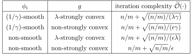
φi g iteration complexityOe(·)
(1/γ)-smooth λ-strongly convex n/m+p(n/m)/(λγ)
(1/γ)-smooth non-strongly convex n/m+p(n/m)/(γ)
non-smooth λ-strongly convex n/m+p(n/m)/(λ)
non-smooth non-strongly convex n/m+pn/m/
Table 1: Iteration complexities of the SPDC method under different assumptions on the functions φi and g. For the last three cases, we solve the perturbed saddle-point
problem with δ=/C1.
The corollary is established by finding the smallestT that satisfies inequality (19).
There are two other cases that can be considered: when φi is not smooth but g is
strongly convex, and whenφi is smooth butg is not strongly convex. They can be handled
with the same technique described above, and we omit the details here. Alternatively, it is possible to use the techniques described in Chambolle and Pock (2011, Section 5.1) to obtain accelerated sublinear convergence rates without using strongly convex perturbations. In Table 1, we list the complexities of the mini-batch SPDC method for finding an-optimal solution of problem (1) under various assumptions. Similar results are also obtained in Shalev-Shwartz and Zhang (2015).
4. SPDC with Non-Uniform Sampling
One potential drawback of the SPDC algorithm is that, its convergence rate depends on a problem-specific constant R, which is the largest `2-norm of the feature vectors ai. As
a consequence, the algorithm may perform badly on unnormalized data, especially if the `2-norms of some feature vectors are substantially larger than others. In this section, we
propose an extension of the SPDC method to mitigate this problem, which is given in Algorithm 3.
The basic idea is to use non-uniform sampling in picking the dual coordinate to update at each iteration. In Algorithm 3, we pick coordinatek with the probability
pk = (1−α)
1
n+α
kakk2
Pn
i=1kaik2
, k= 1, . . . , n, (20)
where α∈(0,1) is a parameter. In other words, this distribution is a (strict) convex com-bination of the uniform distribution and the distribution that is proportional to the feature norms. Therefore, instances with large feature norms are sampled more frequently, con-trolled by α. Simultaneously, we adopt an adaptive regularization in step (21), imposing stronger regularization on such instances. In addition, we adjust the weight of ak in (23)
Algorithm 3:SPDC method with weighted sampling
Input: parametersτ, σ, θ ∈R+, number of iterationsT, initial pointsx(0) and y(0). Initialize: x(0) =x(0),u(0)= (1/n)Pn
i=1y (0)
i ai. for t= 0,1,2, . . . , T−1do
Randomly pickk∈ {1,2, . . . , n}, with probabilitypk given in (20).
Execute the following updates:
yi(t+1) = (
arg maxβ∈R
n
βhai, x(t)i −φ∗i(β)−p2iσn(β−yi(t))2
o
i=k,
y(it) i6=k,
(21)
u(t+1) =u(t)+ 1 n(y
(t+1)
k −y
(t)
k )ak, (22)
x(t+1) = arg min
x∈Rd (
g(x) + D
u(t)+ 1 pk
(u(t+1)−u(t)), x E
+kx−x
(t)k2 2
2τ )
, (23)
x(t+1) =x(t+1)+θ(x(t+1)−x(t)). end
Output: x(T) andy(T).
Theorem 6 Suppose Assumption A holds. Let R := maxikaik2, R := 1nPni=1kaik2 and
Rα := (1−α)/R+α/R
−1
. If the parameters τ, σ, θ in Algorithm 3 are chosen such that
τ = 1
2Rα
r γ
nλ, σ =
1 2Rα
s nλ
γ , θ= 1−
n
1−α +Rα
r n
λγ
−1
, (24)
then for each t≥1, we have
1
2τ +λ
Ekx(t)−x?k22
+
1
4σ + γ n
Eky(t)−y?k22
≤ θt
1
2τ +λ
kx(0)−x?k22+
1
2σ + γ 1−α
ky(0)−y?k22
.
Note that Rα ≤ R/α always holds. If we choose α = 1/2, then the contraction ratio
θ is bounded by 1− n
1−α+ 2R
q
n λγ
−1
. Comparing this bound with Theorem 1 with
m = 1, the convergence rate of Theorem 6 is determined by the average norm of the features, R = n1 Pn
i=1kaik2, instead of the largest one R = maxikaik2. This difference
makes Algorithm 3 more robust to unnormalized feature vectors. For example, if the ai’s
are sampled i.i.d. from a multivariate normal distribution, then maxi{kaik2} almost surely
goes to infinity asn→ ∞, but the average norm 1nPn
i=1kaik2 converges toE[kaik2].
Since θ is a bound on the convergence factor, we would like to make it as small as possible. Letρ:=R/R−1. The expression ofθ in (24) can be minimized by choosing
α? = (
0 ifρ≤pn/κ,
ρ1/2(κ/n)1/4−1
ρ1/2(κ/n)1/4+ρ ifρ > p
where κ = R2/(λγ) is the condition number. The value of α? will be equal to zero if the condition number is large enough, and increases slowly to one as the condition number increases. Thus, we choose a (more conservative) uniform distribution for ill-conditioned problems, but a more aggressively weighted distribution for well-conditioned problems.
For simplicity of presentation, we described in Algorithm 3 a weighted sampling SPDC method with single dual coordinate update, i.e., the case ofm= 1. In fact, the non-uniform sampling scheme can also be extended to mini-batch SPDC. For mini-batch sizem >1, we randomly pick a subset of indices K ⊂ {1,2, . . . , n}of size m. The probability of i∈K is denoted by pi and should satisfy the constraint:
minn1, m1−α
n +
αkaik2
nR o
≤ pi ≤ 1 (26)
fori= 1, . . . , n, and
n
X
i=1
pi =m.
This constraint can be satisfied by first adding all indices {i: pi = 1} to the set K, then
sampling without replacement from the remaining indices in order to make|K|=m. More concretely, there is an efficient sampling-without-replacement algorithm (Chao, 1982) which adds each remaining indexito the setK with probability proportional to 1−nα +αkaik2
nR . It
can be verified that the lower bound in (26) holds with such a procedure.
For the mini-batch extension, we replace the updates (21)-(23) by the following updates:
yi(t+1) = (
arg maxβ∈R
n
βhai, x(t)i −φ∗i(β)− pin
2σm(β−y
(t)
i )2
o
i∈K,
y(it) i /∈K,
u(t+1) =u(t)+ 1 n
X
k∈K
(y(kt+1)−yk(t))ak,
x(t+1) = arg min
x∈Rd
(
g(x) + *
u(t)+ 1 n
X
k∈K
yk(t+1)−yk(t) pk
ak, x
+
+kx−x
(t)k2 2
2τ )
,
which resembles the updates of Algorithm 2. Similar to the mini-batch SPDC, we are able to show that by increasing the batch size m, the convergence rate of the algorithm will be improved. On the other hand, the lower bound onpi given by constraint (26) implies that
with a proper choice of α (e.g.α= 1/2), the convergence rate will depend on
max n
R, m
nR o
,
instead of the maximum normR. Form= 1, we have max{R,mnR}=R, so that it captures the theoretical guarantee for Algorithm 3 as a special case. We omit the proof details.
5. Related Work
Chambolle and Pock (2011) considered a class of convex optimization problems with the following saddle-point structure:
min
x∈Rd
max
y∈Rn
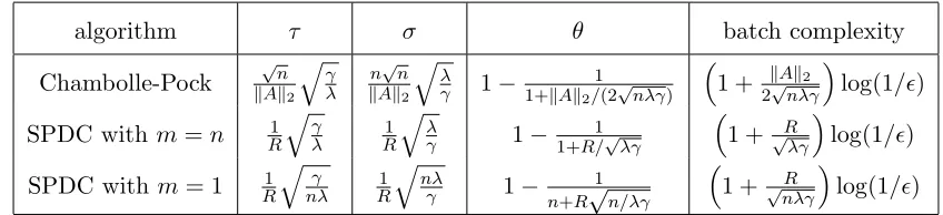
algorithm τ σ θ batch complexity
Chambolle-Pock
√
n
kAk2 q
γ λ
n√n
kAk2 q
λ
γ 1−
1 1+kAk2/(2
√
nλγ)
1 + kAk2
2√nλγ
log(1/)
SPDC withm=n R1
q
γ λ
1
R
q
λ
γ 1−
1 1+R/√λγ
1 +√R
λγ
log(1/)
SPDC withm= 1 R1
q
γ nλ
1
R
q
nλ
γ 1−
1
n+R√n/λγ
1 +√R
nλγ
log(1/)
Table 2: Comparing step sizes and complexity of SPDC with Chambolle and Pock (2011, Algorithm 3, Theorem 3). Here A ∈ Rn×d and its spectral norm kAk
2 usually
grows withn, but always bounded by √nR.
where K ∈ Rm×d, G and F∗ are proper closed convex functions, with F∗ itself being the
conjugate of a convex function F. They developed the following first-order primal-dual algorithm:
y(t+1) = arg max
y∈Rn
hKx(t), yi −F∗(y)− 1
2σky−y
(t)k2 2
, (28)
x(t+1) = arg min
x∈Rd
hKTy(t+1), xi+G(x) + 1
2τkx−x
(t)k2 2
, (29)
x(t+1) =x(t+1)+θ(x(t+1)−x(t)). (30)
When both F∗ and G are strongly convex and the parameters τ, σ and θ are chosen appropriately, this algorithm obtains accelerated linear convergence rate (Chambolle and Pock, 2011, Theorem 3).
We can map the saddle-point problem (4) into the form of (27) by lettingA= [a1, . . . , an]T
and
K= 1
nA, G(x) =g(x), F
∗(y) = 1
n
n
X
i=1
φ∗i(yi). (31)
The SPDC method developed in this paper can be viewed as an extension of the batch method (28)-(30), where the dual update step (28) is replaced by a single coordinate up-date (5) or a mini-batch upup-date (9). However, in order to obtain accelerated convergence rate, more subtle changes are necessary in the primal update step. More specifically, we introduced the auxiliary variable u(t) = n1 Pn
i=1y (t)
i ai = KTy(t), and replaced the primal
update step (29) by (6) and (10). The primal extrapolation step (30) stays the same. To compare the batch complexity of SPDC with that of (28)-(30), we use the following facts implied by Assumption A and the relations in (31):
kKk2 = 1
nkAk2, G(x) is λ-strongly convex, and F
∗(y) is (γ/n)-strongly convex.
The batch complexity of the Chambolle-Pock algorithm isOe(1 +kAk2/(2
√
nλγ)), where theOe(·) notation hides the log(1/) factor. We can bound the spectral norm kAk2 by the Frobenius normkAkF and obtain
kAk2 ≤ kAkF ≤√nmax
i {kaik2}=
√
nR.
(Note that the second inequality above would be an equality if the columns of A are nor-malized.) So in the worst case, the batch complexity of the Chambolle-Pock algorithm becomes
e
O1 +R/pλγ=Oe 1 +
√
κ
, where κ=R2/(λγ),
which matches the worst-case complexity of the accelerated gradient methods (Nesterov, 2004, 2013); see Section 1.1 and also the discussions in Lin et al. (2015b, Section 5). This is also of the same order as the complexity of SPDC with m=n (see Section 2.1). When the condition number κ 1, they can be √n worse than the batch complexity of SPDC withm= 1, which is Oe(1 +
p κ/n).
If either G(x) or F∗(y) in (27) is not strongly convex, Chambolle and Pock (2011, Section 5.1) proposed variants of the primal-dual batch algorithm to achieve accelerated sublinear convergence rates. It is also possible to extend them to coordinate update methods for solving problem (1) when eitherφ∗i orgis not strongly convex. Their complexities would be similar to those in Table 1.
Our algorithms and theory can be readily generalized to solve the problem of
minimize
x∈Rd 1 n
n
X
i=1
φi(ATi x) +g(x),
where eachAiis andi×dmatrix, andφi :Rdi →Ris a smooth convex function. This more general formulation is used, e.g., in Shalev-Shwartz and Zhang (2015). Most recently, Lan and Zhou (2015) considered the case with di = d and Ai =Id, which corresponding to a
general class of problems with the finite-sum (or finite-average) structure. He extended the primal-dual algorithm by replacing the quadratic penalty terms in (5) and (21) with the Bregman divergence associated with the loss functions themselves. This led to an algorithm that does not rely on computing the proximal mapping of the conjugateφ?i, but only requires computing the primal gradient ∇φi at a particular sequence of the primal variables. As a
result, the algorithm in Lan and Zhou (2015) can be considered as a (primal-only or dual-free) randomized incremental gradient algorithm, which share the same order of iteration complexity as SPDC.
5.1 Dual Coordinate Ascent Methods
We can also solve the primal problem (1) via its dual:
maximize
y∈Rn
D(y) def= 1 n
n
X
i=1
−φ∗i(yi)−g∗
−1
n
n
X
i=1
yiai
, (32)
where g∗(u) = supx∈Rd{x
Tu−g(x)} is the convex conjugate of g. Due to the problem
gradient methods for solving this problem (e.g., Platt, 1999; Chang et al., 2008; Hsieh et al., 2008; Shalev-Shwartz and Zhang, 2013a). In the stochastic dual coordinate ascent (SDCA) method a dual coordinate yi is picked at random during each iteration and
up-dated to increase the dual objective value. Shalev-Shwartz and Zhang (2013a) showed that the iteration complexity of SDCA is O((n+κ) log(1/)), which corresponds to the batch complexityO((1 +κ/n) log(1/)).
For more general convex optimization problems, there is a vast literature on coordinate descent methods; see, e.g., the recent overview by Wright (2015). In particular, the work of Nesterov (2012) on randomized coordinate descent sparked a lot of recent activities on this topic. Richt´arik and Tak´aˇc (2014) extended the algorithm and analysis to composite convex optimization. When applied to the dual problem (32), it becomes one variant of the SDCA algorithm studied in Shalev-Shwartz and Zhang (2013a). Mini-batch and distributed versions of SDCA have been proposed and analyzed in Tak´aˇc et al. (2013) and Yang (2013) respectively. Non-uniform sampling schemes similar to the one used in Algorithm 3 have been studied for both stochastic gradient and dual coordinate ascent methods (e.g., Needell et al., 2016; Xiao and Zhang, 2014; Zhao and Zhang, 2015; Qu et al., 2015).
Shalev-Shwartz and Zhang (2013b) proposed an accelerated mini-batch SDCA method which incorporates additional primal updates than SDCA, and bears some similarity to our mini-batch SPDC method. They showed that its complexity interpolates between that of SDCA and accelerated gradient methods by varying the mini-batch size m. In particular, for m =n, it matches that of the accelerated gradient methods (as SPDC does). But for m = 1, the complexity of their method is the same as SDCA, which is worse than SPDC for ill-conditioned problems.
In addition, Shalev-Shwartz and Zhang (2015) developed an accelerated proximal SDCA method which achieves the same batch complexity Oe 1 +
p
κ/n as SPDC. Their method is an inner-outer iteration procedure, where the outer loop is a full-dimensional accelerated gradient method in the primal spacex∈Rd. At each iteration of the outer loop, the SDCA
method (Shalev-Shwartz and Zhang, 2013a) is called to solve the dual problem (32) with customized regularization parameter and precision. In contrast, SPDC is a straightforward single-loop coordinate optimization methods. Two recent works extended the inner-outer iteration method to derive more general accelerated proximal-point algorithms: Frostig et al. (2015) and Lin et al. (2015a). Basically, one can replace the inner-loop SDCA algorithm by other efficient algorithms such as Prox-SVRG (Xiao and Zhang, 2014) or SAGA (Defazio et al., 2014) to obtain the same overall complexity.
More recently, Lin et al. (2015b) developed an accelerated proximal coordinate gradient (APCG) method for solving a more general class of composite convex optimization problems. When applied to solve the dual problem (32), APCG enjoys the same batch complexity
e
5.2 Other Related Work
Another way to approach problem (1) is to reformulate it as a constrained optimization problem
minimize 1
n
n
X
i=1
φi(zi) +g(x) (33)
subject to aTi x=zi, i= 1, . . . , n,
and solve it by ADMM type of operator-splitting methods (e.g., Lions and Mercier, 1979; Boyd et al., 2010). In fact, as shown in Chambolle and Pock (2011), the batch primal-dual algorithm (28)-(30) is equivalent to a pre-conditioned ADMM or an inexact Uzawa method (see, e.g., Zhang et al., 2011). Several authors (Wang and Banerjee, 2012; Ouyang et al., 2013; Suzuki, 2013; Zhong and Kwok, 2014) have considered a more general formulation than (33), where eachφi is a function of the whole vectorz∈Rn. They proposed online or stochastic versions of ADMM which operate on only oneφi in each iteration, and obtained
sublinear convergence rates. However, their cost per iteration isO(nd) instead of O(d). Suzuki (2014) considered a problem similar to (1), but with more complex regularization functiong, meaning thatgdoes not have a simple proximal mapping. Thus primal updates such as step (6) or (10) in SPDC and similar steps in SDCA cannot be computed efficiently. He proposed an algorithm that combines SDCA (Shalev-Shwartz and Zhang, 2013a) and ADMM, and showed that it has linear rate of convergence under similar conditions as Assumption A. It would be interesting to see if the SPDC method can be extended to their setting to obtain accelerated linear convergence rate.
6. Efficient Implementation with Sparse Data
During each iteration of the SPDC method, the update of primal variables (i.e., computing x(t+1)) requires full d-dimensional vector operations; see the step (6) of Algorithm 1, the step (10) of Algorithm 2 and the step (23) of Algorithm 3. So the computational cost per iteration is O(d), and this can be too expensive if the dimension d is very high. In this section, we show how to exploit problem structure to avoid high-dimensional vector operations when the feature vectorsai are sparse. We illustrate the efficient implementation
for two popular cases: whengis an squared-`2 penalty and whengis an`1+`2 penalty. For
both cases, we show that the computation cost per iteration only depends on the number of non-zero components of the feature vector.
6.1 Squared `2-Norm Penalty
Suppose that g(x) = λ2kxk2
2. For this case, the updates for each coordinate of x are
inde-pendent of each other. More specifically, x(t+1) can be computed coordinate-wise in closed form:
x(jt+1)= 1 1 +λτ(x
(t)
j −τ u
(t)
j −τ∆uj), j= 1, . . . , n, (34)
where ∆udenotes (yk(t+1)−yk(t))akin Algorithm 1, or m1 Pk∈K(y
(t+1)
k −y
(t)
k )akin Algorithm 2,
Although the dimension dcan be very large, we assume that each feature vector ak is
sparse. We denote by J(t) the set of non-zero coordinates at iterationt, that is, if for some indexk∈K picked at iterationtwe haveakj 6= 0, thenj∈J(t). If j /∈J(t), then the SPDC
algorithm (and its variants) updatesy(t+1) without using the value of xj(t) orx(jt). This can be seen from the updates in (5), (9) and (21), where the value of the inner producthak, x(t)i
does not depend on the value of x(jt). As a consequence, we can delay the updates on xj
and xj whenever j /∈J(t) without affecting the updates ony(t), and process all the missing
updates at the next time whenj ∈J(t).
Such a delayed update can be carried out very efficiently. We assume that t0 is the last
time when j ∈ J(t), and t
1 is the current iteration where we want to update xj and xj.
Since j /∈J(t) implies ∆uj = 0, we have
xtj+1 = 1 1 +λτ(x
(t)
j −τ u
(t)
j ), t=t0+ 1, t0+ 2, . . . , t1−1. (35)
Notice that u(jt) is updated only at iterations where j ∈ J(t). The value of u(jt) doesn’t change during iterations [t0+ 1, t1], so we haveu(jt) ≡uj(t0+1) fort∈[t0+ 1, t1]. Substituting
this equation into the recursive formula (35), we obtain
x(t1)
j =
1
(1 +λτ)t1−t0−1 x
(t0+1)
j +
u(t0+1) j
λ !
−u (t0+1) j
λ . (36)
The update (36) takes O(1) time to compute. Using the same formula, we can compute x(t1−1)
j and subsequently compute x
(t1)
j = x
(t1) j +θ(x
(t1)
j −x
(t1−1)
j ). Thus, the
computa-tional complexity of a single iteration in SPDC is proporcomputa-tional to|J(t)|, independent of the dimensiond.
We note that similar tricks of delayed updates, or “just-in-time” updates, have been derived and used for the SAG algorithm (Schmidt et al., 2013). For SPDC, the delayed updates become more complex due to the full vector extrapolation required for Nesterov-type acceleration.
6.2 (`1+`2)-Norm Penalty
Suppose thatg(x) =λ1kxk1+λ22kxk22. Since both the`1-norm and the squared`2-norm are
decomposable, the updates for each coordinate ofx(t+1)are independent. More specifically,
x(jt+1)= arg min
α∈R
(
λ1|α|+
λ2α2
2 + (u
(t)
j + ∆uj)α+
(α−x(jt))2 2τ
)
, (37)
where ∆uj follows the definition in Section 6.1. Ifj /∈J(t), then ∆uj = 0 and equation (37)
can be simplified as
x(jt+1) =
1 1+λ2τ(x
(t)
j −τ u
(t)
j −τ λ1) ifx(jt)−τ u
(t)
j > τ λ1, 1
1+λ2τ(x
(t)
j −τ u
(t)
j +τ λ1) ifx(jt)−τ u
(t)
j <−τ λ1,
0 otherwise,
Similar to the approach of Section 6.1, we delay the update of xj until j ∈ J(t). We
assume t0 to be the last iteration when j ∈J(t), and let t1 be the current iteration when
we want to update xj. During iterations [t0+ 1, t1], the value of u(jt) doesn’t change, so we
have u(jt) ≡ u(t0+1)
j for t ∈ [t0 + 1, t1]. Using equation (38) and the invariance of u(jt) for
t∈[t0+ 1, t1], we have an O(1) time algorithm to calculatex(jt1). More specifically, given
x(t0+1)
j at iteration t0, we present an efficient algorithm for calculating x
(t1)
j . We begin by
examining the sign ofx(t0+1)
j .
Case I (x(t0+1)
j = 0): If−u
(t0+1)
j > λ1, then equation (38) impliesx
(t)
j >0 for allt > t0+1.
Consequently, we have a closed-form formula forx(t1) j :
x(t1)
j =
1
(1 +λ2τ)t1−t0−1
x(t0+1)
j +
u(t0+1)
j +λ1
λ2
−u (t0+1)
j +λ1
λ2
. (39)
If−u(t0+1)
j <−λ1, then equation (38) impliesx(jt)<0 for allt > t0+ 1. Therefore, we have
the closed-form formula:
x(t1)
j =
1
(1 +λ2τ)t1−t0−1
x(t0+1)
j +
u(t0+1)
j −λ1
λ2
−u (t0+1)
j −λ1
λ2
. (40)
Finally, if −u(t0+1)
j ∈[−λ1, λ1], then equation (38) implies x(jt1) = 0. Case II (x(t0+1)
j > 0): If −u
(t0+1)
j ≥ λ1, then it is easy to verify that x
(t1)
j is obtained
by equation (39). Otherwise, We use the recursive formula (38) to derive the latest time t+ ∈[t
0+ 1, t1] such that xt
+
j >0 is true. Indeed, since x
(t)
j >0 for all t∈[t0+ 1, t+], we
have a closed-form formula forxtj+:
xtj+ = 1
(1 +λ2τ)t
+−t 0−1
x(t0+1)
j +
u(t0+1)
j +λ1
λ2
−u (t0+1)
j +λ1
λ2
. (41)
We look for the largest t+ such that the right-hand side of equation (41) is positive, which is equivalent of
t+−t0−1<log
1 + λ2x
(t0+1) j
u(t0+1)
j +λ1
/log(1 +λ2τ). (42)
Thus,t+is the largest integer in [t
0+ 1, t1] such that inequality (42) holds. Ift+=t1, then
x(t1)
j is obtained by (41). Otherwise, we can calculatex t++1
j by formula (38), then resort to
Case I or Case III, treatingt+ ast 0.
Case III (x(t0+1)
j < 0): If −u
(t0+1)
j ≤ −λ1, then x(jt1) is obtained by equation (40).
Otherwise, we calculate the largest integert−∈[t0+ 1, t1] such that xt
−
j <0 is true. Using
the same argument as for Case II, we have the closed-form expression
xtj− = 1
(1 +λ2τ)t
−−t
0−1
x(t0+1)
j +
u(t0+1)
j −λ1
λ2
− u (t0+1)
j −λ1
λ2
wheret− is the largest integer in [t0+ 1, t1] such that the following inequality holds:
t−−t0−1<log
1 + λ2x
(t0+1) j
u(t0+1)
j −λ1
/log(1 +λ2τ). (44)
Ift−=t1, thenx(jt1)is obtained by (43). Otherwise, we can calculatext
−+1
j by formula (38),
then resort to Case I or Case II, treating t− ast0.
Finally, we note that formula (38) implies the monotonicity ofx(jt)(t=t0+1, t0+2, . . .).
As a consequence, the procedure of either Case I, Case II or Case III is executed for at most once. Hence, the algorithm for calculatingx(t1)
j hasO(1) time complexity.
The vector x(t1)
j can be updated by the same algorithm since it is a linear combination
of x(t1) j and x
(t1−1)
j . As a consequence, the computational complexity of each iteration in
SPDC is proportional to |J(t)|, independent of the dimensiond.
7. Experiments
In this section, we compare the basic SPDC method (Algorithm 1) with several state-of-the-art algorithms for solving problem (1). They include two batch-update algorithms: the accelerated full gradient (AFG) method (Nesterov, 2004, Section 2.2), and the limited-memory quasi-Newton method L-BFGS (Nocedal and Wright, 2006, Section 7.2)). For the AFG method, we adopt an adaptive line search scheme (Nesterov, 2013) to improve its efficiency. For the L-BFGS method, we use the memory size 30 as suggested by Nocedal and Wright (2006, Section 7.2).
We also compare SPDC with three stochastic algorithms: the stochastic average gradient (SAG) method (Le Roux et al., 2012; Schmidt et al., 2013), the stochastic dual coordinate descent (SDCA) method (Shalev-Shwartz and Zhang, 2013a) and the accelerated stochastic dual coordinate descent (ASDCA) method(Shalev-Shwartz and Zhang, 2015). We conduct experiments on a synthetic dataset and three real datasets. The hyper-parametersτ, σ, θ of the SPDC algorithm are chosen by their theoretical values given in (12). For SDCA, we use their default parameter settings given in Shalev-Shwartz and Zhang (2013a), which can be determined from the Lipschitz constant 1/γ of the loss functions and the strongly convex regularization parameterλ. For SAG, we choose the learning rateα =γ/Ras recommended by Schmidt et al. (2013).
Number of Passes
20 40 60 80
Log Loss
-15 -10 -5 0
AFG L-BFGS SAG SDCA ASDCA SPDC
Number of Passes
50 100 150
Log Loss
-15 -10 -5 0
AFG L-BFGS SAG SDCA ASDCA SPDC
(a) λ= 10−3 (b)λ= 10−4
Number of Passes
100 200 300
Log Loss
-10 -5 0
AFG L-BFGS SAG SDCA ASDCA SPDC
Number of Passes
100 200 300
Log Loss
-4 -3 -2 -1 0
AFG L-BFGS SAG SDCA ASDCA SPDC
(c)λ= 10−5 (d)λ= 10−6
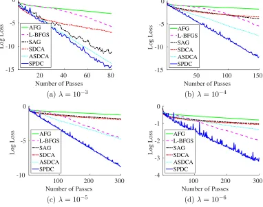
Figure 1: Comparing SPDC with other methods for ridge regression on synthetic data, with the regularization coefficient λ ∈ {10−3,10−4,10−5,10−6}. The horizontal axis is the number of passes through the entire dataset, and the vertical axis is the logarithmic gap log(P(x(T))−P(x?)).
7.1 Ridge Regression with Synthetic Data
We first compare SPDC with other algorithms on a simple quadratic problem using synthetic data. We generaten= 500 i.i.d. training examples {ai, bi}ni=1 according to the model
b=ha, x∗i+ε, a∼ N(0,Σ), ε∼ N(0,1),
where a ∈ Rd and d = 500, and x∗ is the all-ones vector. To make the problem
ill-conditioned, the covariance matrix Σ is set to be diagonal with Σjj =j−2, for j= 1, . . . , d.
Given the set of examples{ai, bi}ni=1, we then solved a standard ridge regression problem
minimize
x∈Rd
(
P(x) def= 1 n
n
X
i=1
1 2(a
T
ix−bi)2+
λ 2kxk
2 2
)
.
In the form of problem (1), we haveφi(z) =z2/2 andg(x) = (1/2)kxk22. As a consequence,
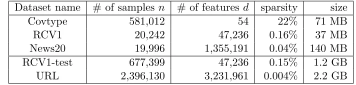
Dataset name # of samples n # of featuresd sparsity size
Covtype 581,012 54 22% 71 MB
RCV1 20,242 47,236 0.16% 37 MB
News20 19,996 1,355,191 0.04% 140 MB
RCV1-test 677,399 47,236 0.15% 1.2 GB
URL 2,396,130 3,231,961 0.004% 2.2 GB
Table 3: Characteristics of real datasets from LIBSVM data (Fan and Lin, 2011).
We evaluate the algorithms by the logarithmic optimality gap log(P(x(t))−P(x?)),
where x(t) is the output of the algorithms after t passes over the entire dataset, and x? is the global minimum. When the regularization coefficient is relatively large, e.g.,λ= 10−1 or 10−2, the problem is well-conditioned and we observe fast convergence of the stochastic algorithms SAG, SDCA, ASDCA and SPDC, which are substantially faster than the two batch methods AFG and L-BFGS.
Figure 1 shows the convergence of the five different algorithms when we varied λ from 10−3 to 10−6. As the plot shows, when the condition number is greater than n, the SPDC algorithm also converges substantially faster than the other two stochastic methods SAG and SDCA. It is also notably faster than L-BFGS. These results support our theory that SPDC enjoys a faster convergence rate on ill-conditioned problems. In terms of their batch complexities, SPDC is up to √n times faster than AFG, and (λn)−1/2 times faster than
SAG and SDCA.
Theoretically, ASDCA enjoys the same batch complexity as SPDC up to a multiplicative constant factor. Figure 1 shows that the empirical performance of SPDC is substantially faster that of ASDCA for small λ. This may due to the fact that ASDCA follows an inner-outer iteration procedure, which requires careful selection of the regularization parameter and accuracy to reach for each call of SDCA. SPDC is a single-loop algorithm that needs less parameters to set up, thus it can be empirically more efficient.
7.2 Binary Classification with Real Data
Finally we show the results of solving the binary classification problem on real datasets. The datasets are obtained from the LIBSVM data collection (Fan and Lin, 2011) and summarized in Table 3. The first three datasets are selected to reflect different relations between the sample sizenand the feature dimensionality d, which cover nd(Covtype), n ≈ d (RCV1) and n d (News20). The remaining two are relatively larger datasets (RCV1-test and URL) that we did not test in previous experiments conducted in Zhang and Xiao (2015). For all tasks, the data points take the form of (ai, bi), where ai ∈ Rd is the feature vector, and bi ∈ {−1,1} is the binary class label. As a preprocessing step, the
feature vectors are normalized to the unit`2-norm (meaningR= 1).
Our goal is to minimize the regularized empirical risk:
P(x) = 1 n
n
X
i=1
φi(aTi x) +
λ 2kxk
2
2, where φi(z) =
0 ifbiz≥1
1
2 −biz ifbiz≤0 1
Here,φi is the smoothed hinge loss (see, e.g., Shalev-Shwartz and Zhang, 2013a). It is easy
to verify that the conjugate function of φi is φ∗i(β) = biβ+ 12β2 for biβ ∈ [−1,0] and ∞
otherwise.
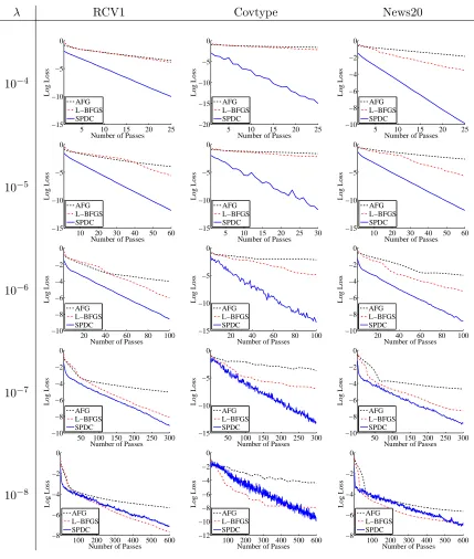
The performance of the five algorithms on the three smaller datasets are plotted in Figure 2 and Figure 3. In Figure 2, we compare SPDC with the two batch methods: AFG and L-BFGS. The results show that SPDC is substantially faster than AFG and L-BFGS for relatively large λ, illustrating the advantage of stochastic methods over batch methods on well-conditioned problems. Asλdecreases to 10−8, the batch methods (especially L-BFGS) become comparable to SPDC.
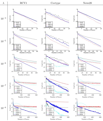
In Figure 3, we compare SPDC with the three stochastic methods: SAG, SDCA and ASDCA. Note that the specification of ASDCA (Shalev-Shwartz and Zhang, 2015) requires the regularization coefficientλsatisfiesλ≤ 10R2n whereRis the maximum`2-norm of feature
vectors. To satisfy this constraint, we run ASDCA withλ∈ {10−6,10−7,10−8}. In Figure 3, the observations are just the opposite to that of Figure 2. All stochastic algorithms have comparable performances on relatively large λ, but SPDC and ASDCA becomes substan-tially faster when λgets closer to zero. In particular, ASDCA converges faster than SPDC on the Covtype dataset, but SPDC is faster on the remaining two datasets. In addition, due to the outer-inner loop structure of the ASDCA algorithm, its error rate oscillates and might be bad at early iterations. In contrast, the curve of SPDC is almost linear and it is more stable than ASDCA.
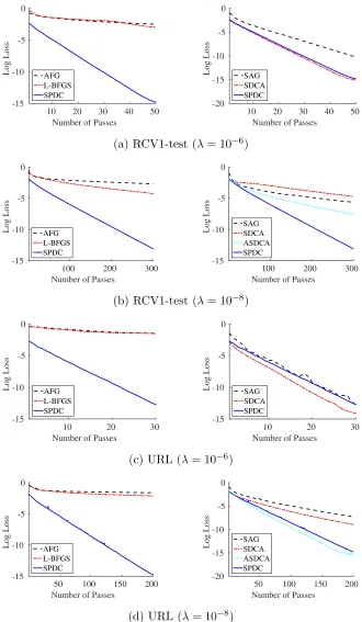
Figure 4 plots the convergence results on the last two datasets, where both the sample size n and the dimension d are big. If the regularization parameter λ is also relatively large, then the stochastic algorithms (SPDC, SAG and SDCA) will guarantee to converge very quickly, making it an easy optimization problem. We report experiments on small regularization values λ = 10−6 and λ = 10−8. The ASDCA algorithm is reported on λ = 10−8 because it satisfies the constraint λ ≤ R2
10n. Comparing results on the RCV1
and RCV1-test datasets, the SPDC algorithm has a more significant advantage over the batch methods (AFG and L-BFGS) on the bigger dataset, because the stochastic algorithm converges faster with a larger sample size. On the other hand, the performance gaps between SPDC and the two other stochastic methods (SAG and SDCA) are less significant on the bigger dataset. We observe the same phenomenon on the URL dataset.
Summarizing Figure 2, Figure 3 and Figure 4, the performance of the SPDC algorithm are always comparable or better than the other methods, for various of relations between the sample size nand the dimensiond, and on both small and large datasets.
7.3 Uniform Sampling versus Non-Uniform Sampling
In this subsection, we compare the uniform sampling strategy (Algorithm 1) and the non-uniform sampling strategy (Algorithm 3) for SPDC. We repeat the binary classification experiments on the Covtype, RCV1 and News20 datasets, but this time without performing feature normalization. More precisely, for each data point taking the form of (ai, bi), we
don’t normalize the feature vector ai to the unit `2-norm. But instead, we multiply a
constant number to every feature vector so that the average `2-normR is equal to one. It
λ RCV1 Covtype News20
10−4
5 10 15 20 25 −15
−10 −5 0
Number of Passes
Log Loss
AFG L−BFGS SPDC
5 10 15 20 25 −20
−15 −10 −5 0
Number of Passes
Log Loss
AFG L−BFGS SPDC
5 10 15 20 25 −10 −8 −6 −4 −2 0
Number of Passes
Log Loss
AFG L−BFGS SPDC
10−5
10 20 30 40 50 60 −15
−10 −5 0
Number of Passes
Log Loss
AFG L−BFGS SPDC
5 10 15 20 25 30 −15
−10 −5 0
Number of Passes
Log Loss
AFG L−BFGS SPDC
10 20 30 40 50 60 −15
−10 −5 0
Number of Passes
Log Loss
AFG L−BFGS SPDC
10−6
20 40 60 80 100 −10 −8 −6 −4 −2 0
Number of Passes
Log Loss
AFG L−BFGS SPDC
20 40 60 80 100 −15
−10 −5 0
Number of Passes
Log Loss
AFG L−BFGS SPDC
20 40 60 80 100 −10 −8 −6 −4 −2 0
Number of Passes
Log Loss
AFG L−BFGS SPDC
10−7
50 100 150 200 250 300 −10 −8 −6 −4 −2 0
Number of Passes
Log Loss
AFG L−BFGS SPDC
50 100 150 200 250 300 −15
−10 −5 0
Number of Passes
Log Loss
AFG L−BFGS SPDC
50 100 150 200 250 300 −10 −8 −6 −4 −2 0
Number of Passes
Log Loss
AFG L−BFGS SPDC
10−8
100 200 300 400 500 600 −8
−6 −4 −2 0
Number of Passes
Log Loss
AFG L−BFGS SPDC
100 200 300 400 500 600 −12 −10 −8 −6 −4 −2 0
Number of Passes
Log Loss
AFG L−BFGS SPDC
100 200 300 400 500 600 −8
−6 −4 −2 0
Number of Passes
Log Loss
AFG L−BFGS SPDC
λ RCV1 Covtype News20
10−4
5 10 15 20 25 −15
−10 −5 0
Number of Passes
Log Loss
SAG SDCA SPDC
5 10 15 20 25 −20
−15 −10 −5 0
Number of Passes
Log Loss
SAG SDCA SPDC
5 10 15 20 25 −15
−10 −5 0
Number of Passes
Log Loss
SAG SDCA SPDC
10−5
10 20 30 40 50 60 −15
−10 −5 0
Number of Passes
Log Loss
SAG SDCA SPDC
5 10 15 20 25 30 −15
−10 −5 0
Number of Passes
Log Loss
SAG SDCA SPDC
10 20 30 40 50 60 −15
−10 −5 0
Number of Passes
Log Loss
SAG SDCA SPDC
10−6
Number of Passes
20 40 60 80 100
Log Loss -10 -5 0 SAG SDCA ASDCA SPDC
Number of Passes
20 40 60 80 100
Log Loss -20 -15 -10 -5 0 SAG SDCA ASDCA SPDC
Number of Passes
20 40 60 80 100
Log Loss -10 -5 0 SAG SDCA ASDCA SPDC 10−7
Number of Passes
100 200 300
Log Loss -10 -5 0 SAG SDCA ASDCA SPDC
Number of Passes
100 200 300
Log Loss -15 -10 -5 0 SAG SDCA ASDCA SPDC
Number of Passes
100 200 300
Log Loss -10 -5 0 SAG SDCA ASDCA SPDC 10−8
Number of Passes
200 400 600
Log Loss -8 -6 -4 -2 0 SAG SDCA ASDCA SPDC
Number of Passes
200 400 600
Log Loss -10 -5 0 SAG SDCA ASDCA SPDC
Number of Passes
200 400 600
Log Loss -8 -6 -4 -2 0 SAG SDCA ASDCA SPDC
Number of Passes
10 20 30 40 50
Log Loss
-15 -10 -5 0
AFG L-BFGS SPDC
Number of Passes
10 20 30 40 50
Log Loss
-20 -15 -10 -5 0
SAG SDCA SPDC
(a) RCV1-test (λ= 10−6)
Number of Passes
100 200 300
Log Loss
-15 -10 -5 0
AFG L-BFGS SPDC
Number of Passes
100 200 300
Log Loss
-15 -10 -5 0
SAG SDCA ASDCA SPDC
(b) RCV1-test (λ= 10−8)
Number of Passes
10 20 30
Log Loss
-15 -10 -5 0
AFG L-BFGS SPDC
Number of Passes
10 20 30
Log Loss
-15 -10 -5 0
SAG SDCA SPDC
(c) URL (λ= 10−6)
Number of Passes
50 100 150 200
Log Loss
-15 -10 -5 0
AFG L-BFGS SPDC
Number of Passes
50 100 150 200
Log Loss
-20 -15 -10 -5 0
SAG SDCA ASDCA SPDC
(d) URL (λ= 10−8)
Number of Passes
100 200 300 400 500
Log Loss
-8 -6 -4 -2 0
Uniform-SPDC Non-Uniform-SPDC
Number of Passes
100 200 300 400 500
Log Loss
-15 -10 -5 0
Uniform-SPDC Non-Uniform-SPDC
Number of Passes
100 200 300 400 500
Log Loss
-8 -6 -4 -2 0
Uniform-SPDC Non-Uniform-SPDC
(a) RCV1 (R/R= 3.87) (b) Covtype (R/R= 1.25) (c) News20 (R/R= 6.71)
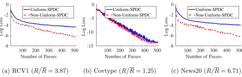
Figure 5: Comparing the uniform sampling and non-uniform sampling strategies for SPDC, where the vertical axis is the logarithmic optimality gap log(P(x(t))−P(x?)). The quantityR/R represents the ratio between the largest feature norm and the average feature norm. When this quantity is large, the non-uniform sampling algorithm converges significantly faster.
For this experiment, we use a small regularization parameter λ = 10−8, so that the problem has a large condition number. The hyper-parameters τ, σ, θ are chosen by their theoretical values in (12) and (24), respectively for the two sampling strategies. For non-uniform sampling, the hyper-parameter α is chosen by the optimal value given in (25). Figure 5 plots their convergence profiles. On all of the three datasets, the non-uniform sampling algorithm converges faster. The margin is quite significant when the ratio between the largest feature norm R and the average feature norm R is relatively large. This is consistent with our analysis in Theorem 1 and Theorem 6, which state that the convergence rate of the uniform sampling algorithm dependsR, while that of the non-uniform sampling algorithm depends on R.
Acknowledgments
We are grateful to Qihang Lin for helpful discussions, especially on the proof of Lemma 3.
Appendix A. Proof of Theorem 1
We focus on characterizing the values of xand y after the t-th update in Algorithm 2. For any i∈ {1, . . . , n}, let yei be the value of y
(t+1)
i ifi∈K, i.e.,
e
yi= arg max β∈R
βhai, x(t)i −φ∗i(β)−
(β−yi(t))2 2σ
.
Since by assumptionφi is (1/γ)-smooth, its convex conjugate φ∗i isγ-strongly convex (see,