A Direct Path to Intelligent Tools
-60- Abstract — A computer application designed to generalize linear elements in a vector formatted cartographic set by means of two of the most contrasted line generalization algorithms, Douglas-Peucker simplification and Bézier curves based smoothing, is presented in this paper. Regarding codification, the simultaneous treatment of different lineal geometry entity classes and the conservation of their original topological relationships among them are considered. It is recommended in processes that produce small scale reductions (in a 1:2 relationship or similar). The application allows changing the characteristic parameters of the referred algorithms and proposes a report of the results obtained after every transformation. That way it supplies an additional facility as a trial tool to choose the parameters that give the best results in every process.
Keywords — Geographic information system, linear features, map generalization, simplification, smoothing, topological relationships.
I. INTRODUCTION
artography is a graphic expression mean whose main function consists in transmitting information (geographic, in this case) and in helping to understand it. In order to achieve this double aim, the map has to maintain the equilibrium between the clarity of the information, its richness, and the exactitude in its localization. So the cartographer affronts two fundamental questions: on the one hand the affluence of information presented by the geographic reality obliges to select the elements to be represented; on the other hand, its dimensions impose a reduction to make them comprehensible, which implies a greater accumulation of adjacent elements, a growing complexity in forms, and, in general, a loss of clarity [1]. These two issues selection and reduction require a set of transformations that preserve the rigor of the results. The whole of these transformations conforms the so called cartographic generalization process
[2], that intervenes in a decisive way in the basic (from direct observations) and derived (from the latter through scale reduction) cartographic production. In short, generalization is a natural process and it is necessary when building a map [1], so that both concepts are intimately related [3].
The cartographic generalization process must ensure the following essential requirements:
1.Achievement of a suitable positional exactitude.
2.Implementation of a treatment of the set of different entity classes that preserves their mutual topological relationships. 3.Allowance for the study of the goodness of the obtained
results.
The numerous efforts dedicated to the research of the automation of the process, all of them based in geographical information systems technology (GIS), have permitted to dispose today of specific commercial programs of generalization («Radius Clarity» of the British firm 1Spatial; «CTP», of the Institute of Cartography and Geomatics of Leibniz University in Hannover, Germany) and generalization modules or tools in existing GIS programs. In general, these solutions propose methodologies for the application of different algorithms of generalization and present the following characteristics:
They establish a semiautomatic process of generalization using a set of automatic operations that must be completed afterwards with a manual treatment.
They are oriented to the generalization of geometry elements or concrete characteristics: contour lines, communication routes, built-up areas, etc.
They treat geographic information in an independent way, without considering it in its whole and within the geographic context in which it finds itself. Therefore they do not keep topological relationships (intersections, inclusions, etc.) among the different entity classes, even among the elements of the same class. All in all the resulting set losses geometric consistency, global sense and, in many cases, harmony with respect to the original.
They do not produce reports of the obtained results, which makes difficult the analysis of its goodness. These characteristics allow the conclusion that, regarding the three already mentioned essential requirements of the generalization process, every available solutions assure the first one, some of them take into account partially the second one, and none of them the third one, which suggests the elaboration of a specific computer application to achieve them. On the other hand, most of the mentioned algorithms are meant to achieve the generalization of linear elements in vector format, because the entities that make up a map are represented mainly through lines and polygons, and these are limited by lines [4]. According to Thapa [5] they are approximately the 80% of the elements in a cartographic representation. In order to generalize these elements, one of the solutions that provide best results consists of simplifying its geometry (elimination of points) and smoothing afterwards the obtained result. Among the line simplification algorithms, the
Douglas-Peucker algorithm [6] is the best considered for small scale reductions [7]-[8]. Concerning smoothing algorithms, also called «curvature filtering», the ones based on
Béziercurves make one of the most commended alternatives [9]-[10].
A prototype for linear features generalization
C
Wenceslao Lorenzo Romero, Rubén González Crespo, Andrés Castillo Sanz
Pontifical University of Salamanca, Computer Science Faculty, Madrid, Spain.
-61- As a contribution to these researches, in this paper a computer application is presented, which allows to:
Generalize linear elements in vector format so as to obtain small scale reductions (in the 1:2 relationship or similar) by applying the Douglas-Peucker algorithm and the one based on Bézier curves and preserving their mutual topological relationships.
Change characteristic parameters of mentioned algorithms.
Present a report over each one of the applied transformations: number of obtained axes, number initial and final points and processing time.
II.DOUGLAS-PEUCKER ALGORITHM
The Douglas-Peucker algorithm implemented in this application is the second of the line simplification methods presented in 1973 by the Canadian teachers David H. Douglas
(Ottawa) and Thomas K. Peucker (Simon Fraser University, British Columbia) [6]. Besides it is used in most current GIS commercial tools that include generalization tools (ArcInfo from ESRI, GeoMedia Professional from Intergraph or Bentley MicroStation GeoGraphics).
It is based on the treatment as a whole of all the points that compose the geometry of each line. That is the reason why the line simplification algorithms are included under the so called the «global» ones [11].
The fundament of the algorithm consists of selecting in the original line specific points that are called critical or anchor points which will build the generalized line. In order to select them, a tolerance factor de tolerance T > 0 is established beforehand. It is called simply tolerance and is expressed in length units. The process can be resumed in the following steps (see example in figure 1) [1]:
1. Tolerance is set to T > 0.
2. A first segment AZ between initial node A and final one Z on the line is traced.
3. The distances di of the vertices to segment AZ are calculated. If no distance is greater than the tolerance (di < T), the process ends and the generalized line will be composed by points A and Z. On the contrary, if vertex B is more distant from AZ (dimáx = dB), it will be selected as a critical point and two new segments AB y BZ will be generated.
4. The distances d'i of the rest of the intermediate vertices to segments AB and BZ are calculated and the selection procedure from the previous step is applied.
5. This criterion is repeated recursively in the two parts in which the segments are divided after every selection, as far as the division possibilities of the segments are exhausted.
6. Finally, a generalized line is obtained from the selected points in each step.
If the lines are closed, the first and last points do not define a line because A and Z coincide for their having the same coordinates, the maximum distance to initial segment is replaced by the greatest distance to these points. Nevertheless, in this case it is controversial to select as critical point a point
of the curve just for having been digitalized in the first or in the last place.
Fig. 1. Example of the application of de Douglas-Peucker algorithm [1].
Some authors designate as additive this type of simplification algorithms, while the so called subtractive ones remove successively several points in each step [11].
Apart from the simplicity provided by the algorithm, both in its codification and in the simplification process that it sets out, one of its main advantages consists in allowing the positional control of the generalized line with respect to the original one, because the tolerance T determines the greatest displacement between them.
On the other hand, the increase of T affects the obtained result in the following aspects (table I):
Table I. Consequences of the increase of the value of t.
Aspect Variation
Points of the resultant line Diminishes Processing time Diminishes
Smoothing Diminishes
Topological conflicts Increases Adaptations to the original line Diminishes
That is why, it becomes necessary to evaluate the obtained results to achieve in each process the tolerance that would provide equilibrated results in the mentioned aspects.
III. BÉZIER CURVES
-62- shifting [11], Gaussian filtering [13], Boyle [14]), frequency domain (Fourier series, wavelets) and mathematical approximations. Due to the interest of our study, we will center in the third group. Its fundament consists in obtaining an approximation to the original line by adjusting with respect to it some of the plane curves defined by polynomial equations of degree greater than one (circumferences, parables, cubic arcs, etc.). One of the most used methods is the one based on the splines [15], which are curves defined by segments by means of polynomials. Bézier curves make up the base for the best known and most used smoothing algorithms too.
The theoretical fundaments of the Bézier curves were developed by the French engineer Pierre Bézier (1910-1999) during the 60s of last century [16]. These fundaments will be briefly referred next [17].
In the context of linear algebra, the approach to the mentioned adjustment is the following: given a function y = f (x) whose value is known in n + 1 points (P0, P1,... , Pn), and its
value is approximated in an another arbitrary point P. To achieve that, a polynomial of degree less than n which would adopt the known values f (xi) for i = 0, 1, ..., n is used. This is
the so called classic polynomial adjustment or polynomial interpolation problem1. There exist solutions of global adjustment (Lagrange formula, Newton formula) which consider all known data, and solutions of segment adjustment (splines), which interpolate a curve between every two given points.
In the field of graphic design, the parametric equations are the most used for representing curves, due, among other reasons, to the convenience of make independent the definition of the curve from the used coordinate system. In the same trend, the adjustment problems usually are solved beginning from the parametric equations. Centering in our problem and considering in the plane the surface we are interested in the n + 1 points of known coordinates (x0, y0), (x1, y1), ..., (xn,
yn), the obtained curve after the adjustment (global or by
segments), expressed in parametric form, will have this form:
, n nx P t
y Q t
(1)
whereP tn
adjusts the values (ti, xi) and Q tn
adjusts in (ti, xi),being ti= i/n, with i = 0 , 1, ..., n.
This adjustment presents, among others, the inconvenient of not allowing the control of the form of the curve the user is designing. In order to avoid this conflict, one of the most used resources is the Bézier curves, based on the Bernstein polynomials.
The Bernstein polynomials of degree n, called
0,n , 1,n , ..., n n, ,
B t B t B t are defined by the following
expression:
, 1 ,
n i i i n
n
B t t t
i (2)
with i = 0, 1,… , n.
1 Besides this one there exist other adjustment problems (Taylor,
Hermite, etc.) that will not be treated here because they will take far away from the pretentions of this article.
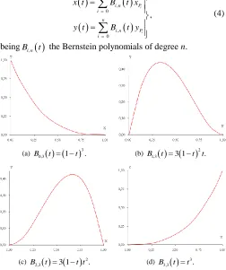
So, for example, the Bernstein polynomials of degree 3 are:
3 2 0,3 1,3 2 3 2,3 3,31 , 3 1
. 3 1 ,
B t t B t t t
B t t t B t t
(3)
In figure 2 its graphic representation can be seen, with t [0, 1]. A Bézier curve associated to n + 1 points of the plane (P0,
P1,... , Pn) is the denomination of the curve defined for t [0,
1] whose parametric equations adopt the following expression:
, 0 , 0 ,
i i ni n P i
n
i n P i
x t B t x
y t B t y
(4)
beingBi n,
t the Bernstein polynomials of degree n.
(a) B0,3
t 1 t
3. (b)
21,3 3 1 .
B t t t
(c)
22,3 3 1 .
B t t t (d)
33,3 .
B t t
Figure 2. Bernstein polynomials of degree 3.
The points P0, P1,... , Pn that determine a Bézier curve are
called control points and, as it can be deduced from expression 4, its order is fundamental: its tracing passes only through initial P0 and final Pn points, while the rest mark its «tendency»
without forming part of it (figure 3). Graphically, this means that the Bézier curve associated to the precedent n + 1 points supposes a smoothed polygonal line formed by these ones. Therefore, in the context of cartographic generalization different smoothing algorithms have appeared which use mathematical approximations based on the Bézier curves.
-63- (a) P0 = (1, 5), P1 = (2, 2),
P2 = (4, 1) y P3 = (5, 3).
(b) P0 = (1, 5), P1 = (2, 2),
P2 = (5, 4) y P3 = (4, 1).
Figura 3. Curvas de Bézier.
As a consequence, in order to use Bézier curves as smoothing algorithm, it is necessary to establish previously the number of values that the mentioned parameter should adopt, considering the following criteria:
The original curve can be smoothed out keeping its tendency starting form a number of values of t equal to the number of points of the curve, which will constitute the control points of the resulting Bézier curves.
The layout of the Bézier curves improves, if well distributed values of t inside the indicated interval are chosen. In table II some examples are included.
Table II. Appropriate values of parameter t in function of the number of control points.
Number of
control points Values of t
3 0 0,50 1
4 0 0,33 0,66 1
5 0 0,25 0,50 0,75 1
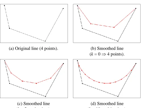
The more the number of values of t are, the more the smoothing effect improves. From now on, k will be the number of values of t added to the number of points of the curve (control points). This growth supposes an increment of points of the final curve and a more laborious calculation process. These issues oblige to evaluate the obtained results to attain an equilibrium solution among the added number of values, the processing time and the aesthetics of the resulting smoothing (figure 4 and table III).
(a) Original line (4 points). (b) Smoothed line (k = 0 4 points).
(c) Smoothed line
(k = 2 6 points).
(d) Smoothed line (k = 10 14 points).
Figure 4. Bézier Curves.
Table III. Appropriate values of parameter t with different values of k (n = 3 4 control points).
k Values of t
0 0 0,33 0,66 1
2 0 0,20 0,40 0,60 0,80 1
10 0 0,08 0,15 0,23 0,31 0,38 0,46 0,54 0,62 0,69 0,77 0,85 0,92 1
At last, the number of control points should be reduced for two main reasons:
1. In the algebraic expression of the Bernstein polynomials (equation 2), on which the Bézier curves are based, each one of the parametric equations x(t) and y(t) includes n + 1 combinatorial numbers that are calculated by means of factorials, being n the number of control points. The calculation capacity of the computer systems limits the number of possible factorials and, in definitive, the number of control points.
2. In this sense, the conditions of obtaining a resulting line adapted as much as possible to the tracing of the original becomes more restrictive. When the number of control points increases, the mean distances between both of them rise up to inacceptable values.
For that reason the criterion of using the so called cubic Bézier curves with four control points was adopted.
IV. GENERAL CHARACTERISTICS OF THE PROGRAM
Next the general characteristics of the application will be presented, as it will detailed afterwards [18]:
It is a command of the GIS application GeoMedia Professional (Intergraph), valid for the last versions (6.0 y 6.1).
The Visual Basic .Net language has been used for its codification, with the development environment Microsoft Visual Studio 2005. Although there exist subsequent versions of that environment (2008 y 2010), the programming of the command require the employment of the complement GeoMedia Command Wizard which at the moment can only be used on 2005 version.
It codes the Douglas-Peucker algorithm and the one based on the Bézier curves aforementioned, allowing the variation of the characteristic tolerance of the first one and the number of points added in the second one.
It admits vector files in .mdb format, which is specific of GeoMedia, generated with the data base manager system Access. They are relational databases (DB) that store the geographic information in tables, so that on each table the elements belonging to the same entity class or to several ones of the same themes are recorded. In a table, each recorded or row corresponds to an element of the class, whose attributes and coordinates are stored in the different fields or columns that constitute the record.
-64-
It permits the treatment as a whole of several entity classes (tables), when they are linear, keeping the topologic relationships among them.
It presents a report on the screen after processing each file and it allows saving in a text file the obtained results.
V.INFORMATION PROCESSING
Once the program is installed and the access from the application is created, the command gets activated when establishing any connection in read-write mode to a DB ( .mdb file). It consists of a main dialogue window with four functionality areas (figure 5):
Fig. 5. Main dialogue window of the generalization command.
1. Table management (in the DB of the established connections).
2. Douglas-Peucker. 3. Bézier.
4. Douglas-Peucker + Bézier.
Two bars centered on the inferior part show the progression in the application of each process: «Progreso Tabla» shows progress of the treatment of each table individually; «Progreso Total» shows the progress of the whole process.
The «Gestión de tablas» area presents the options that are next described:
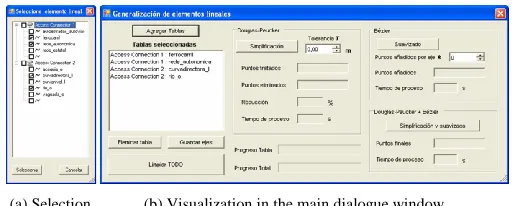
«Agregar Tablas». It shows another dialogue window with the established connections. When deploying them, the tables with the elements of linear geometry that form each connected database come up. The selected tables (figure 6a) are visualized in the main panel after clicking the «Seleccionar» button (figure 6b).
«Eliminar Tabla». It permits to delete one by one any of the tables selected before.
(a) Selection. (b) Visualization in the main dialogue window.
Fig. 6. Selection tables from different DB.
«Guardar ejes». It builds a topology among the elements of the selected tables and it saves the coordinates of the resulting axes in a text file (.txt) (figure 7).
«Limpar TODO». It deletes all the selected tables and the results appear on the windows after any the algorithms is applied.
Fig. 7. Building of the topology: resulting axes are shown.
The «Douglas-Peucker» area allows the application of this algorithm independently. Once the tables are selected in the previous area, it includes the following options:
«Tolerancia T». It permits to select the tolerance in meters.
«Simplificación». It implements the following successive operations:
5. It records the time at which the process. 6. It loads the selected tolerance.
7. It starts the progression bars.
8. It builds up the topology among the elements of the selected tables by cross comparing the tables with one another and with themselves. That way the nodes that make up the crosses among elements are obtained and their position remains the same as it should. Every two consecutive nodes constitute an axis.
9. With each one of the axes, a) It counts the number of points.
b) It applies the algorithm with the selected tolerance, checking before two questions:
1.Whether the initial and final nodes coincide (it is a closed line). In this case, it dispenses with the final node, it applies the algorithm to the rest of the points and finally it adds the final node to the resulting line. 2.Whether it has less than three points, in which case it is not applied and the axis remains invariable.
c) It counts the number of points of the final axis. As it was indicated, the resulting lines keep the initial and final points of the original lines, so that it is guaranteed to conserve the position of the extreme nodes of each axis. 10.After the generalization of every axis, it combines
them to rebuild the geometry of each final line. 11.It saves this geometry by modifying the tables that
contain now the new elements.
12.It records the final instant of the process.
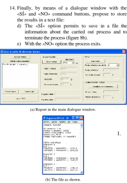
-65- 14.Finally, by means of a dialogue window with the
«SÍ» and «NO» command buttons, propose to store the results in a text file:
d) The «SÍ» option permits to save in a file the information about the carried out process and to terminate the process (figure 8b).
e) With the «NO» option the process exits.
(a) Report in the main dialogue window.
(b) The file as shown.
Fig. 8. Results from the application of the Douglas-Peucker algorithm (T = 5 m).
As regards the «Bézier» area it permits the independent application of the algorithm based on the Bézier curves. Once selected the tables previously in the «Gestión de tablas » area, it includes the following options:
«Puntos añadidos por eje k». It allows the input of the number of points to add by resulting axis, which it has been called k.
«Suavizado». It runs successively the following operations:
1. It records the time at which the process starts. 2. It loads the added points input by axis. 3. It starts the progress bars.
4. It builds up the topology among the elements of the selected tables with the same procedure as in the previous case.
5. With each axis:
f) It counts the number of points. 6. It divides it in segments of four points.
7. It calculates the parametric equations of the resulting Bézier curves considering as control points the four points that make up each segment.
8. It calculates the points of the Bézier curve associated to the four pints of the segment assigning different values to the parameter t. If the value of the «Puntos añadidos por eje» windows is not modified (by default, k = 0), t adopts four values in the [0, 1] interval, so that with t = 0 and t = 1 initial and final points will be the same, respectively,
and the rest of the values are symmetrically distributed in that interval. If a k > 0 value is introduced, the program assigns 4 + k different values for t, which are distributed the criterion above.
The resulting curves keep the same initial and final points of the original lines, according with what has been discussed above. Therefore, the initial topology keeps the same.
9. As in the previous case, after the generalization of every axis, it combines them, rebuilding the geometry of each resulting line and modifying the tables that contain the new elements.
10.It records the finalization time of the process.
11.It calculates the processing time and the total number of added points (k times the number of points obtained in the topologic construction). It presents the results in the respective text boxes of the main dialogue window (figure 9).
12.Besides, once finalized the process, the program proposes to save the results in a text file following the above mentioned procedure.
1.
Fig. 9. Application of the algorithm based on the Bézier curves (k = 1).
Report in the main dialogue window.
As regards the «Douglas-Peucker + Bézier» area, it permits the successive application of both algorithms. Once previously selected the tables in the «Gestión de tablas» area and introduced the values of «Tolerancia T» and the number of «Puntos añadidos por eje k» in the «Douglas-Peucker» and «Bézier» areas, respectively, the «Simplificación y suavizado» option carries out the following sequence of operations:
1. It records the start time of the process. 2. It loads the added points by axis. 3. It loads the selected tolerance. 4. It starts the process bars.
5. It builds up the topology with the same procedure as in the above cases.
6. With each axis:
g) It applies the Douglas-Peucker algorithm, following independently the process.
h) It applies the algorithm based on the Bézier curves, conforming to the independent process.
7. As in the former cases, it combines the transformed axis rebuilding the geometry of every resulting line and modifying the tables that contain the new elements. 8. Likewise, it presents the option of saving the results in a
-66- Fig. 10. Douglas-Peucker Algorhitm (T = 5 m) based on Bezier curves (k = 2).
Report on the main dialog box.
VI. CONCLUSIONS
The described computer application, recommended in processes that suppose small scale reductions (in a 1:2 relationship or similar), offers two main capacities:
1. The generalization of the linear elements of a cartographic set in vector format. In order to attain this, the application codes the Douglas-Peucker simplification algorithm and the smoothing one based on the Bézier curves, considering the simultaneous treatment of different geometry entity classes and preserving the original topological relationships among them.
2. The analysis of the obtained results after the transformation made by the previous process, by means of the trial with different parameters and the contrast of the results. In order to get that, the application permits to change the characteristic parameters of the concerned algorithms and it offers a report of the results after each process: treated, deleted, added or final points, in every case, as well as the processing time.
VII. ACKNOWLEDGMENT
To Captain D. Carlos Borrallo Corisco for his inestimable collaboration in the codification of the program.
REFERENCES
[1] W. Lorenzo, “Generalización automática de curvas de nivel en un proceso de reducción de escala de 1:50000 a 1:100000,” Mapping, nº. 129, pp. 50-64, 2008.
[2] A. H. Robinson and R. D. Sale, Elements of Cartography (3th
ed.). University of Wisconsin, Madison, Alabama, 1969.
[3] J. L. García, “Generalización de elementos lineales mediante algoritmos en el dominio espacial y de la frecuencia,” doctoral thesis, director: F. J. Ariza, Universidad de Jaén, 2006.
[4] A. Skopeliti and L. Tsoulos, “On the parametric description of the shape of the cartographic line,” Cartografica, 36(3), pp. 53-65, 1999. [5] K. Thapa, “Automatic line generalization using zero-crossing,”
Photogrammetric Engineering and Remote Sensing, 56(4), pp.
511-517, 1988.
[6] D. H. Douglas y T. K. Peucker, “Algorithms for the reduction of the number of points required to represent a digitised line or its caricature”,
The Canadian Cartographer, 10(2), pp. 112-122, 1973.
[7] M. Visvalingam and J. D. Whyatt, “The Douglas-Peucker algorithm for line simplification: re-evaluation through visualization,” Computer
Graphics Forum, 9(3), pp. 213-228, 1990.
[8] M. Visvalingam and P. J. Williamson, “Simplification and generalization of large scale data for roads: a comparison of two filtering algorithms,” Cartographic and Geographic Information Systems, 20(2), pp. 96-106, 1995.
[9] D. Nagy, “Generalization and PostScript,” Simposium on Geospatial
Theory, Proccesing and Applications, Ottawa, Canada, 2002.
[10] A. Cecconi, “Integration of cartographic generalization and multi-scale databases for enhanced web mapping,” doctoral thesis, directors: R. Weibel, M. Sester, and D. Burghart,
Mathematisch-naturwissenschaftlichen Fakultät der Universität Zürich, 2003.
[11] R. B. McMaster and S. K. Shea, Generalization in digital cartography. Association of American Cartographers, Washington, D. C., 1992. [12] J. L. García, “Automatización de los procesos de segmentación y
clasificación de vías de comunicación en generalización cartográfica”, doctoral thesis, director: F. J. Ariza, Departamento de Ingeniería Cartográfica, Geodésica y Fotogrametría, Escuela Politécnica Superior,
Universidad de Jaén, 2006.
[13] J. Badaud, A. P. Witkin, M. Baudin and R. O. Duda, “Uniqueness of the Gaussian kernel for scale-spade filtering,” IEEE Transactions on
Pattern Analysis and Machine Intelligence, 8(1), pp. 26-33, 1986.
[14] A. R. Boyle, “The quantised line,” The Cartographical Journal, 7(2): pp. 91-94, 1970.
[15] R. B. McMaster, “Integration of simplification and smoothing algorithms in line generalization,” Cartographica, 26(1), pp. 101-121, 1989.
[16] P. Bézier, “Procédé de définition numérique des courbes et surfaces non mathématiques,” Automatisme¸ XIII (5), pp. 189-196, 1968.
[17] E. A. Lebrón, “Apuntes de ampliación de matemáticas,” Ingeniería Técnica en Diseño Industrial, Departamento de Matemática Aplicada II, Escuela Universitaria Politécnica, Universidad de Sevilla, 2005. [18] C. Borrallo and W. Lorenzo, “Generalización Cartográfica. Comando de
GeoMedia Professional”, tesis final del 29 Curso de Geodesia.
Departamento de Geodesia y Topografía (Escuela de Guerra del
![Fig. 1. Example of the application of de Douglas-Peucker algorithm [1].](https://thumb-us.123doks.com/thumbv2/123dok_us/9718007.1955149/2.612.314.563.84.319/fig-example-application-douglas-peucker-algorithm.webp)