An efficient algorithm for computing two-dimensional discrete cosine transforms

MURDOCH RESEARCH REPOSITORY

http://dx.doi.org/10.1109/ISCAS.1991.176357

Ta, N., Attikiouzel, Y. and Crebbin, G. (1991) An efficient

algorithm for computing two-dimensional discrete cosine

transforms. In: IEEE International Sympoisum on Circuits and

Systems, 11 - 14 June, pp. 396-399.

http://researchrepository.murdoch.edu.au/19981/

Copyright © 1991 IEEE

Personal use of this material is permitted. However, permission to reprint/republish

this material for advertising or promotional purposes or for creating new collective

An

Efficient Algorithm for Computing Two-Dimensional

Discrete Cosine Transforms

Nhi

Ta,

Yianni Attikiouzel and Greg Crebbin

Department

of

Electrical and Electronic Engineering

The University of Western Australia

Nedlands, Western Australia 6009

AUSTRALIA

Abstract

A fast algorithm for computing the two-dimensional discrete cosine transform (2-D DCT) is proposed. In this algorithm the 2-D DCT is converted into a form of 2-D DFT which is called the odd DFT(ODFT). The odd DFT can be calculated by a DFT followed by post-multiplications. The DFT part of odd DFT is calculated by the fast discrete Radon transform.

A brief description of the Gertner method [5] for computing the 2-D FFT is presented in section 2, together with the radix- 2 fast discrete Radon transfrom (FDRT). The mapping used in converting the DCT into an odd DFT, and the 2-D DCT algorithm by using the FDRT are described in section 3. A

discussion on the computational complexity of the algorithm is presented in section 4.

The complexity of the proposed algorithm is comparable t o the

polynomial transform approach. This new algorithm produces

Computing

Of

the

2-D

DFT

a regular structure which makes it attractive for VLSI imple-

mentation. Furthermore, the computation can be performed in parallel.

1

Introduction

Since its introduction in 1974, the discrete cosine transform

[l] has found many applications in image processing, and data compression; due t o its ability t o closely approximate the op- timal Karhunen-Loeve transform (KLT) and its suitability for implementation by a fast algorithm. Recently, it has been adopted by the CCITT as part of the video coding standard.

In image coding, a 2-D DCT is used. The usual way of computing the 2-D DCT has been the row-column approach, where a 2-D DCT of an (NxN) block is decomposed into N DCTs for the N rows and N DCTs for the N columns. Recent studies [7] [4] have shown that direct 2-D techniques are more efficient than row-column approaches.

Most of the direct 2-D methods for computing 2-D DCT are based on polynomial transform [4] [7]. In [4]

,

the polynomial transform is used t o calculated the 2-D FFT and a rotation stage is used t o perform the complex multiplications. In a

recent paper [7], the polynomial transform is performed on the

W$kl term. The latter reduces the computational complexity

a t the expense of a more complex algorithm and flowgraph structure.

In this paper, a 2-D direct computation of the 2-D DCT is proposed. The method is based on the geometric relationship between points on a 2-D grid. The 2-D DCT is first formu- lated as a two-dimensional odd DFT (2-D ODFT). The newly formed 2-D ODFT can be calculated by a 2-D DFT and post-

In this section, we briefly describe the discrete Radon trans- form (DRT) for computing a 2-D DFT proposed by Gertner

[ 5 ] , in order t o understand the computation of the 2-D DCT.

A 2-D DFT is defined as

i=o j=o

where W N = e-3zrr/N, and k , 1 = 0,. . .

,

N - 1.

Gertner [ 5 ] has shown that an (NxN) point 2-D DFT can be computed by taking a number of N-point 1-D DFTs, where this number is equal to the number of linear congruences of the (NxN) grid. For N = 2n, the number of linear congruences on the (NxN) grid is 3N/2.

The 2-D DFT can now be calculated using the following equations:

N - 1

X(< N - ml > ~ , 1 ) = Rl(m,d)WE ( 2 a )

d=O

m = 0 , 1 , . . . , N - 1 1 = 0, I , . . . , N - 1

N-1

X ( k ,

<

N - 2sk > N ) = R2(s,d)Wkd (26)

d=O

s = 0, l , . . . , N/2 - 1 k = 0,1,

’”,

N - 1

where R1 and Rz are the DRTs on the input array z ( i , j ) ,

which are defined as:

Rl(m,d) = N-1 z ( i ,

<

d t mi > N )

d,m = O , . . . , N - 1

N-1

R ~ ( s , d ) = x(< d

t

2si > N , i ) (3b)

i=O

d = O,...,N

-

1 s = O , . . . , N / 2 - 1 Normally, the DRT requires i ( N - 1 ) N 2 additions. A

radix-2 algorithm is used to reduce the number of additions for computing the DRT [6]. Let

2'-1

R f ) ( i , m, d ) = ~ ( j 2 ~ - ~

+

i ,

<

d

+

m(j2n-'

+

i ) > N ) ( 4 ~ )

j=O

2 t - 1

R f ) ( i , s , d ) = z(< d

+

2s(j2n-t

+

i) > ~ , j 2 ~ - ~

+

i) (4b)

for i = 0,. . . ,2n-t - 1. The DRT can be computed in n stages. At each stage 1,

j=O

R E ( i , m , d ) = R r - ' ) ( i , m , d ) + R:-"(i+ 2n-t,m,d)

Ri(i, s, d ) = R:-')(i, s, d )

+

R!-')(i

+

2n-t, s, d )

( 5 a )

(5b)

where

R y ) ( i , m, d ) = ~ ( i ,

<

d

+

mi > N )

R P ) ( i , s , d ) = x ( < d + 2 s i > ~ , i ) ( 6 b )

R l ( m , d ) = Rp)(O, m , d )

R2(s, d ) = Rp)(O, s, d )

( s a )

and

( 7 a )

( 7 a )

By using the following properties:

RF'(i, m

+

# , d ) = R f ) ( i , m,

<

d

+

iq2t > N ) ( s a )

( 8 h )

RF)(i, s

t

$?-',

d ) = R f ) ( i , s ,

<

d

+

i# > N )

the ranges of m and s in each stage t , reduces t o m = 0 , .

.

.

,

2t - 1 and s = 0,. , ,

,

2t-1 - 1. Hence, the number of additions re-

quired to compute the DRT for an (NxN) array, where N = 2n,

is

4

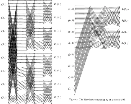
l o g ( N ) N 2 . The flowgraph of FDRT for an ( 8 x 8) array is shown in Figures 2 and 3, for RI and R2 respectively. Note that the second stage for R2 is the same as the two blocks in the second stage of RI. As we can see, the structure of the flowgraph is very regular. This feature makes the FDRT approach for computing 2-D FFT easily adaptable for VLSI implementation.

3

Computing

2-D

DCT using FDRT

In this section, we describe the mapping that enables the com- putation of a DCT via a DFT. A 1-D DCT is defined as follows:

2 4 %

+-

1)k 4N N - l

X ( k ) = x(i)cos

i=O

(9)

k = 0 , 1 , . . . , N - 1 By using the classical mapping [2], [3]

the DCT becomes

k = O , l , . . . , N - 1

Using a trigonometric identity, the expression for X ( N - k) is similar t o the above equation except that the cosine function is replaced by a sine function. Hence we can define a transform

U ( k ) as follows:

N-1

(12)

U ( k ) = X ( k )

+

j X ( N -

k)

= y ( i ) W 4 , (4i+l)k

i=O

Note that we only need t o evaluate k such that the set {k, N

-

k } = (0,.

. .

,

N - 1).

For the 2-D case, the 2-D DCT is defined as:

k,Z = 0 , . . ., N - 1

By analogy with the 1-D case, it is easy t o recognize that the 2-D DCT coefficients can be obtained from U ( k , 1 ) by the following set of equations :

X ( k , Z ) = R e [ U ( k , Z ) + j U ( N

-

k,Z)]

(14) X ( k , N - Z ) = - I m [ U ( k , Z ) $ j U ( N - k , 1 ) ] X ( N

-

k,Z) = - I m [ U ( k , Z ) - j U ( N - k , 1 ) ]

X ( N - k , N - l ) = - R e [ U ( k , l ) - j U ( N - k , Z ) ]

~

i=O j = O

and y ( i , j ) is the 2-D extension of the mapping described in equation (10). [4]

i = 0 , . . ., N / 2

-

1

j = 0,. .

.,

N / 2 - 1

i = N / 2 ,

...,

N - 1

i = O ,

...,

N / 2 - 1

j = N / 2 ,

...,

N - 1

x ( 2 N - 2i - l , 2 j )

x ( 2 i , 2N - 2j - 1 )

j = 0,. . ., N / 2 - 1

Y(i,j) =

(16)

Note that eqn (14) requires U ( k , l ) t o be computed for all

k,

and only a subset of Z such that

{Z,

N -

Z}

cover all possible values of 1.

We can rewrite U ( k , 1 ) as follows:

i = O j = O

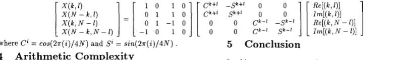
We observe that the summation in the above equation is identical t o that for the 2-D DFT. This can be calculated us- ing the FDRT approach, the post-multiplication stage can be implemented as suggested in 141:

1 0 ck+l X ( k ,

4

X ( N - 6 , N - 1)

[

$2;;

j

=

[

-;

i

-;

;

j

[

""0"

0

where C' = cos(2?r(i)/4N) and S' = sin(2x(i)/4N) .

4

Arithmetic Complexity

Let the M[.] and A[.] denote the number of multiplications and additions needed t o compute [.] respectively. Since the algorithm can be divided into two stages, the DFT and post- multiplications. The number of multiplications and additions required for the FDRT-based 2-D DFT for real ( N x N ) array are respectively:

7

6 M[DFT(N x N)] = 1og(N)N2/2 - - N 2 t 8/3

A[DFT(N x N)] = 310g(N)N2 - 2N2

+

18

The number of multiplication and addition for the post multi- plication stage are (3N2-2N) and (5N2-6N+2) respectively. Hence, the number of multiplications and additions required for 2-D DCT of a ( N x N ) array are:

11

6

M[DCT(N x N)] = 1og(N)N2/2

+

-N2 - 2N t 8/3

A[DCT(N x N)] = 310g(N)N2

+

3N2 - 6N

+

20 The measure of computation complexity of the proposed al- gorithm is shown in Table 1 together with that of other algo- rithms for comparison. The complexity of the proposed ap- proach is comparable with the current polynomial transform methods. The number of multiplications is the same as for

the Vetterli approach, and greater than that for the Duhamel- Guillemot. The number of additions are generally slightly more than that of the polynomial transform methods. A reduc- tion in the number of additions can be achieved by examining

In this paper we proposed a new method for computing the 2-D DCT using a number of 1-D DFTs which is less than 2N. The measure of arithmetic complexity is comparable with the other approaches in the current literature. Research in this area should be able to reduce the complexity even further. The flowgraph of the proposed algorithm has regular struc- ture which can be easily implemented using VLSI. Finally, the algorithm is well suited for parallel implementation.

References

[l] N. Ahmed, T. Natarajan, and K.R. Rao, "Discrete Cosine Transform," IEEE Trans. Comp., vol C-23, pp 90-93, 1974. [2] M.J. Narasimha and A.M. Peterson, "On the computation of

the discrete cosine transform," IEEE Trans. Comm., vol COM-

26, pp 934936, 1978.

(31 M . Vetterli and H.J. Nussbaumer, "Simple FFT and DCT algc- rithms with reduced number of operations," Signal Processing,

vol6, pp 267-278, 1984.

[4] M . Vetterli, "Fast 2-D Discrete Cosine Transform", Proc. IEEE

ICASSP'85 pp 1538-1541, 1985.

[5] I. Gertner, "A new efficient algorithm to compute the twc- dimensional discrete Fourier transform," IEEE Trans. Acous.

Speech Szg. Proc., vol ASSP-36, pp 1036-1050, 1988.

[6] D. Yang, "Fast Discrete Radon Transform and 2-D Discrete Fourier Transform," Elec. Lett., vol26, no 8, pp 550-551, 1990. [7] P. Duhamel and C. Guillemot "Polynomial Transform Compu- tation of the 2-D DCT," Proc. IEEE ICASSP'SO, pp 1515-1518, 1990

the redundancies in the computing of the FDRT, for example,

Rz(0,O) = Rl(0,O).

N-FFT

N-FFT _{Back Mapping}

Figure 3: The Flowchart computing R2 of a 8 x 8 FDRT

Polynomial Polynoiiiial Proposed N Transform [7] Transform [4] Algorithm Mult. Add. Mult. Add. Mult. Add. 8 96 484 104 462 104 580 16 512 2531 568 2558 568 3124 32 2560 12578 2840 12950 2840 15700 64 12288 60578 13528 62442 13528 75412 Figure 2: The flowchart for computing R1 of a 8 x 8 fast discrete

Radon transform

row-col F F C T [3]

Mult. Add. 192 464 1024 2592 5120 13376 24576 65664

Table 1: Arithmetic coinplexity of NxN 2-D D C T algorithms.